VESIcal: An open-source thermodynamic model engine for mixed volatile (H₂O-CO₂) solubility in silicate melts
Abstract
Thermodynamics has been fundamental to the interpretation of geologic data and modeling of geologic systems for decades. However, more recent advancements in computational capabilities and a marked increase in researchers’ accessibility to computing tools has outpaced the functionality and extensibility of currently available modeling tools. Here we present VESIcal (Volatile Equilibria and Saturation Identification calculator): the first comprehensive modeling tool for H2O, CO2, and mixed (H2O-CO2) solubility in silicate melts that: a) allows users access to seven of the most popular models, plus easy inter-comparison between models; b) provides universal functionality for all models (e.g., functions for calculating saturation pressures, degassing paths, etc.); c) can process large datasets (1,000’s of samples) automatically; d) can output computed data into an Excel spreadsheet or CSV file for simple post-modeling analysis; e) integrates plotting capabilities directly within the tool; and f) provides all of these within the framework of a python library, making the tool extensible by the user and allowing any of the model functions to be incorporated into any other code capable of calling python. The tool is presented within this manuscript, which may be read as a static PDF but is better experienced via the Jupyter notebook version of this manuscript. We present here worked examples accessible to python users with a range of skill levels. The basic functions of VESIcal can also be accessed via a web app (https://
Key Points
- The first comprehensive volatile solubility tool capable of processing large datasets automatically
- Seven built-in solubility models, with automatic calculation and plotting functionality
- Built in python and easily usable by scientists with any level of coding skill
Plain Language Summary
Geologists use numerical models to understand and predict how volcanoes behave during storage (pre-eruption), eruption, and the composition and amount of volcanic gas released into the atmosphere of Earth and other planets. Most models are made by performing experiments on a limited dataset and creating a model that applies to that dataset. Some models combine lots of these individual models to make a generalized model that can apply to lots of different volcanoes. Many of these different models exist, and they all have specific uses, limitations, and pitfalls. Here we present the first tool, VESIcal, which acts as a simple interface to seven of the most commonly used models. VESIcal is written in python, so users can use VESIcal as an application or include it in their own models. VESIcal is the first tool that allows geologists to model thousands of data points automatically and provides a simple platform to compare results from different models in a way never before possible.
1Introduction
Understanding the solubility and degassing of volatiles in silicate melts is a crucial component of modeling volcanic systems. As dissolved components, volatiles (primarily H2O and CO2) affect magma viscosity, rheology, and crystal growth. In addition, due to the strong dependence of volatile solubility on pressure, measured volatile concentrations in preserved high-pressure melts (i.e., melt inclusions: liquid magma trapped within crystals at high pressure, then brough to the surface during an eruption) can be used to determine pre-eruptive magmatic storage pressures, and thus depths. Importantly, volatile exsolution-driven overpressure of a magmatic system is likely the trigger of many explosive volcanic eruptions Tait et al., 1989Blake, 1984Stock et al., 2016. Once triggered, further drops in magmatic pressure caused by ascent of magma within a volcanic conduit result in the continuous exsolution of volatiles from the melt. Volatile elements experience a large positive volume change when moving from a dissolved to exsolved free fluid state. This expansion fuels a dramatic increase in the magma’s buoyancy, which can often lead to a runaway effect in which the ascent and degassing of volatile-bearing magma eventually erupts at the surface in an explosive fashion. Working in concert with seismic and gas monitoring data, pre-eruptive magmatic volatile concentrations as well as solubility and degassing modelling can be used in forensic and sometimes in predictive scenarios, helping us to understand and potentially mitigate the effects of explosive eruptions.
All of these processes depend directly on the solubility – or the capacity of a magma to hold in solution – of volatile elements. Over the last several decades, a veritable explosion of new volatile solubility data has opened the door to a plethora of models describing the solubility of H2O, CO2, or mixed H2O-CO2 fluid in magmas covering a wide compositional, pressure, and temperature range. Volatile solubility is highly dependent upon the composition of the host magma, making already challenging experiments more onerous to perform to encapsulate the range of magmas seen in nature. The most fundamental models Stolper, 1982Dixon et al., 1995Moore et al., 1998 focus on a specific range of magma bulk compositions (e.g., basalt or rhyolite only). Later studies filled in compositional gaps, some with an increased focus on mixed-volatile (H2O-CO2) studies, increasing the natural applicability of our models to more systems Liu et al., 2005Iacono-Marziano et al., 2012Iacovino et al., 2013. To date, there have been only a few significant efforts to create a holistic thermodynamic model calibrated by a wide range of data in the literature. The most popular are MagmaSat (the mixed-volatile solubility model built into the software package MELTS v. 1.2.0; Ghiorso & Gualda (2015)) and the model of Papale et al. (2006). Both of these studies have made their source code available; the Papale et al. (2006) FORTRAN source code (titled Solwcad), web app, and a Linux program can be found at http://
Despite this communal wealth of solubility models, quantitative calculations of volatile solubility, and by extension saturation pressures, equilibrium fluid compositions, and degassing paths, remains a time-consuming endeavor. Modeling tools that are available are typically unable to process more than one sample at a time, requiring manual entry of the concentrations of 8-10 major oxides, temperature, as well as CO2 and H2O concentrations to calculate saturation pressures, or X to calculate dissolved volatile contents. This is particularly problematic for melt inclusion studies, where saturation pressures are calculated for hundreds of inclusions, each with different entrapment temperatures, CO2, H2O, and major element concentrations. For example, the saturation pressures from 105 Gakkel ridge melt inclusions calculated in MagmaSat by Bennett et al. (2019) required the manual entry of 1,365 values! The potential for user error in this data entry stage should not be overlooked.
In many cases, newly published solubility models do not include an accompanying tool, requiring users to correctly combine and interpret the relevant equations e.g., Dixon et al., 1995Dixon, 1997Liu et al., 2005Shishkina et al., 2014. This is problematic from a perspective of reproducibility of the multitude of studies utilizing these models, especially given that some of the equations in the original manuscripts contain typos or formatting errors. For some models, an Excel spreadsheet was provided, or available at request from the authors. For example, Newman & Lowenstern (2002) included a simplified version of the Dixon (1997) model as part of “VolatileCalc”, which was written in Visual Basic for Excel. Due to its simplicity, allowing users to calculate saturation pressures, degassing paths, isobars and isopleths with a few button clicks and pop-up boxes, this tool has proved extremely popular (with 836 citations at the time of writing). However, to calculate saturation pressures using VolatileCalc, the user must individually enter the SiO2, H2O, CO2 content and temperature of every single sample into pop-up boxes. Similarly, the Excel spreadsheet for the Moore et al. (1998) model calculates dissolved H2O contents based on the concentration of 9 oxides, temperature, and the fraction of X in the vapor, which must be pasted in for every sample. Finally, Allison et al. (2019) provide an Excel spreadsheet that allows users to calculate fugacities, partial pressures, isobars, isopleths and saturation pressures. Again, parameters for each sample must be entered individually, with no way to calculate large numbers of samples automatically.
Some of these published models and tools are at risk of being lost to time, since spreadsheet tools (particularly earlier studies published before journal-provided hosting of data and electronic supplements was commonplace) must be obtained by request to the author. Even if the files are readily available, programs used to open and operate them may not support depreciated file formats. More recently, authors have provided web-hosted interfaces to calculating saturation pressures and dissolved volatile contents (e.g., Iacono-Marziano et al. (2012); http://
While we certainly advocate for the continued refinement of solubility models, including the completion of new experiments in poorly studied yet critical compositional spaces such as andesites Wieser et al., 2021, a perhaps more crucial step at this juncture is in the development of a tool that can apply modern computational solutions to making our current knowledge base of volatile solubility in magmas accessible and enduring.
Here we present VESIcal (Volatile Equilibria and Saturation Identification calculator): a python-based thermodynamic volatile solubility model engine that incorporates seven popular volatile solubility models under one proverbial roof. The models included in VESIcal are (also see Table 1):
- MagmaSat: VESIcal’s default model. The mixed-volatile solubility model within MELTS v. 1.2.0 Ghiorso & Gualda, 2015
- Dixon: The simplification of the Dixon (1997) model as implemented in VolatileCalc Newman & Lowenstern, 2002
- DixonWater and DixonCarbon available as pure-fluid models
- MooreWater: (Moore et al. (1998); water only, but H2O fluid concentration can be specified)
- Liu: Liu et al., 2005
- LiuCarbon and LiuWater available as pure-fluid models
- IaconoMarziano: Iacono-Marziano et al., 2012
- IaconoMarzianoWater and IaconoMarzianoCarbon available as pure-fluid models
- ShishkinaIdealMixing: Shishkina et al., 2014 using pure-H2O and pure-CO2 models and assuming ideal mixing. In general, the pure-fluid versions of this model should be used
- ShishkinaWater and ShishkinaCarbon available as pure-fluid models
- AllisonCarbon: Allison et al., 2019, carbon only
- AllisonCarbon_vesuvius (default; phonotephrite from Vesuvius, Italy)
- AllisonCarbon_sunset (alkali basalt from Sunset Crater, AZ, USA)
- AllisonCarbon_sfvf (basaltic andesite from San Francisco Volcanic Field, AZ, USA)
- AllisonCarbon_erebus (phonotephrite from Erebus, Antarctica)
- AllisonCarbon_etna (trachybasalt from Etna, Italy)
- AllisonCarbon_stromboli (alkali basalt from Stromboli, Italy)
As any individual model is only valid within its calibrated range (see below), and each model is parameterized and expressed differently (e.g., empirical vs. thermodynamic models), it is impractical to simply combine them into one large model. Instead, VESIcal is a single tool that can access and utilize all built-in models, giving VESIcal an extensive pressure-temperature-composition calibration range Figure 1. VESIcal is capable of performing a wide array of calculations on large datasets automatically, with built-in functionality for extracting data from an Excel or CSV file. In addition, the code is written such that it is flexible (sample, calculation type, and model type can be chosen discreetly) and extensible (VESIcal code can be imported for use in python scripts, and the code is formatted such that new volatile models can be added).
Importantly, VESIcal has been designed for practicality and ease of use. It is designed to be used by anyone, from someone who is completely unfamiliar with coding to an adept programmer. The non-coder user can interact with VESIcal through a webapp (https://10.5281/zenodo.5095382) for the current version of the code, along with a snapshot of the GitHub repository at the time of release.
A detailed history of volatile solubility modeling and the implications of VESIcal are explored in detail in the companion manuscript to this work, Wieser et al. (2021).
2Research Methodology
Navigating the array of models implemented in VESIcal can be challenging. How can a user determine which model best suits their needs? MagmaSat (the default model in VESIcal) is the most widely calibrated in P-T-X space, and so we recommend it for the majority of cases. Where a user wishes to use the other implemented models, we provide some tools to help choose the most appropriate model (see Supplement). These tools are described in more detail in Section 3.4 on comparing user data to model calibrations.
Table 1:Calibration ranges of VESIcal models
| Model/Reference | Species | P (bar) | T (°C) | Compositional range | Notes |
|---|---|---|---|---|---|
| MagmaSat Ghiorso and Gualda, 2015 | H2O | 0–20,0001 | 550-14201 | Very broad compositional range of natural silicate melts: subalkaline picrobasalts to rhyolites, including a variety of mafic and silicic alkaline compositions | 1Ranges extracted from Fig. 2d of Ghiorso and Gualda. 2015 |
| CO2 | 0–30,0001 | 1139-14001 | |||
| H2O - CO2 | 0–10,0001 | 800-14001 | |||
| Dixon Simplification of Dixon (1997) used in VolatileCalc (Newman and Lowenstern, 2002) | H2O - CO2 | 0-50001 0-20002 0-10003 | 600-15001 (1200)4 | Alkali basalts: 40-49 wt% SiO2 | 1Warnings implemented in VolatileCalc (Newman and Lowenstern, 2002). 2Calibration range suggested by Lesne et al. (2011) 3Calibration range suggested by Iacono-Marziano et al. (2012) 4Calibration temperature of Dixon (1997) |
| MooreWater Moore et al. 1998 | H2O | 0–30001 | 700–12001 | Broad compositional range: subalkaline basalts to rhyolites, alkaline trachybasalts-andesites, foidites, phonolites | 1Author-suggested calibration range. The calibration dataset spans 190 to 6067 bar, and 800-1200°C |
| Liu Liu et al. 2005 | H2O - CO2 | 0-50001 | 700–12001 | Haplogranites and rhyolites | 1Author-suggested calibration range for the mixed fluid model. The calibration dataset covers 750-5510 bar and 800-1150°C for the Carbon model, and 1-5000 bar and 700-1200 °C for the water model |
| Iacono-Marziano Iacono-Marziano et al., 2012 | H2O - CO2 | 95–10,500 (mostly <5000)1 | 1100-1400 (preferably 1200- 1300)2 | Predominantly mafic compositions: subalkaline and alkaline basalts-andesites | 1Range of calibration dataset, as authors do not specifically state a calibration range. We note that the vast majority of experiments were conducted at <5000 bar. 2Authors state that most experiments were conducted between 1200-1300°C (whole range 1100-1400°C |
| Shishkina Shishkina et al. 2014 | H2O1 | 0–50002 | 1050–1400 (preferably 1150- 1250)2, 3 | Mafic and intermediate compositions: Subalkaline basalts- basaltic andesites, alkali basanites-phonolites. SiO2<65 wt%. | 1Although their empirical expressions are for pure fluids, they were mostly calibrated on mixed CO2-H2O experiments. 2Author-suggested range 3Note, this model contains no temperature term. |
| CO21 | 500–50002 | 1200–12502, 3 | Predominantly mafic compositions: subalkaline basalts, alkaline basanites, trachybasalts | ||
| AllisonCarbon Allison et al., 2019 | CO2 | 0-70001 | 12002 (~1000-1400) | Alkali-rich mafic magmas from six volcanic fields. Separate model coefficients for each composition. | 1Author-suggested range. The calibration dataset spans: (SFVF: 4133–6141 bar, Sunset Crater: 4071-6098 bar, Erebus: 4078-6175 bar, Vesuvius: 269-6175 bar, Etna=485-6199, Stromboli=524-6080) 2Note, all calculations performed at 1200°C (the experimental temperature). Authors suggest results generally applicable between 1000-1400°C |

Figure 1:Illustrations showing the calibrated ranges of VESIcal models in pressure-temperature space. Due to difficulty in differentiating between pure-CO2 and mixed fluid experiments in the literature, plots are subdivided into: experiments performed with pure-CO2 or mixed (H2O-CO2) fluid; and pure-H2O fluid.
A list of model names recognized by VESIcal can be retrieved by executing the command v.get_model_names(), assuming VESIcal has been imported as v as is demonstrated in worked examples below. Note that the model names as listed in the previous section are given in terms of how to call them within VESIcal (e.g., model='MooreWater'). Allison et al. (2019) provides unique model equations for each of the six alkali-rich mafic magmas investigated in their study. The default model in VESIcal is that calibrated for Vesuvius magmas, whose calibration has the widest pressure range of the study Table 1. Setting a model name of 'AllisonCarbon' within VESIcal will thus result in calculations using the AllisonCarbon_vesuvius model equations.
All of the calculations implemented in VESIcal can be performed using any of the models included. The code is structured by calculation rather than by model, which provides an intuitive way for users to interact with the code and compare outputs from multiple models. Each calculation class is instantiated with the model name and any applicable data as arguments. It then performs five key functions: 1) creates the requested model object and performs any necessary pre-processing (e.g., ensuring relevant data are present; normalizing data); 2) takes user input and performs the mathematical calculation; 3) does any necessary processing of the output (e.g., normalizing totals); 4) checks that the model is being used within its calibrated range; and 5) stores calculated outputs in an intuitive and manipulatable format (e.g., a python dictionary, a figure, or a pandas DataFrame). Results of calculations can be saved to one or more Excel or CSV files. To demonstrate that VESIcal returns results which are comparable with pre-existing tools, we have performed a number of tests, which are described in the Supplementary Information (Text S2). For single-sample calculations, the calculation object has the following attributes that can be called by the user: model_name, sample (both provided by the user), model (an instance of the Model class used to run the calculations of interest), result (the result of the calculations), and calib_check (the results of the calibration check).
2.1Model Calibrations and Benchmarking
The pressure, temperature, and composition calibration ranges of the seven models implemented in VESIcal are shown in Table 1 and Figure 1. VESIcal abides by statements of caution made by the authors of these models regarding their extrapolation by informing the user if a calculation is being performed outside of a model’s calibrated range. In this case, the code returns a warning message, which is as specific as possible, along with the requested output. We also provide several Jupyter notebooks in the supplementary material (Supplementary Text S3-S4 and Supplementary files S1-S7), allowing users to plot their data amongst the calibrations of the different models to assess their suitability for less objective measures. Detailed descriptions of the seven solubility models implemented in VESIcal, including information about their calibration range in terms of melt composition, pressure, and temperature, are given in Wieser et al. (2021)
Testing was undertaken to ensure that VESIcal faithfully reproduces the results of all incorporated models. When possible, all models were benchmarked by testing VESIcal outputs against those of a relevant published calculator (e.g., web apps or Excel macros). The models of Shishkina et al. (2014) and Liu et al. (2005) were published with no such tool and so testing instead compares VESIcal outputs to experimental conditions or analyses and, where possible, plots VESIcal results against published figures. All models underwent multiple tests, the results of which are shown in the supplement (Supplementary Text S3-S4 and Supplemental Jupyter Notebooks S1-S7). For all models, VESIcal reproduced the results from previous tools (e.g., web apps, Excel spreadsheets) to within ±1% relative and often on the order of ±0.1% relative.
MagmaSat, VESIcal’s default model, underwent three tests, the results of which are shown in Figure 2: 1. Comparison of saturation pressures from MORB melt inclusions in VESIcal to those published by Bennett et al. (2019), who used the MagmaSat Mac App (R2=0.99998; Figure 2a); 2. Comparison of fluid composition (X) calculated with VESIcal and the web app (R2=0.999, identical considering the web app returns 2dp; Figure 2b); 3. Comparison of isobars for the Early Bishop Tuff calculated with VESIcal (star symbols) and isobars published in Figure 14 of Ghiorso & Gualda (2015) (Figure 2c). VESIcal outputs using the model of Dixon (1997) were tested against outputs from the VolatileCalc Excel spreadsheet Newman & Lowenstern, 2002 and a widely used Excel macro e.g., Tucker et al., 2019.

Figure 2:Benchmarking of VESIcal against MagmaSat. a. Comparison of saturation pressures calculated with VESIcal against those by Bennett et al. (2019) using the MagmaSat app for Mac. Samples are all MORB melt inclusions, and pressures were calculated at a temperature unique to each sample. b. Equilibrium fluid compositions calculated with VESIcal against those calculated with the MagmaSat web app. c. Individual points along the 1,000, 2,000, and 3,000 bar isobars for the Early Bishop Tuff rhyolite calculated with VESIcal (stars) and plotted atop isobars published in Figure 14 of Ghiorso & Gualda (2015).
2.2Format of the python library
In this section, the basic organization and use cases of VESIcal are discussed. VESIcal relies heavily on python pandas, a python package designed for working with tabulated data. Knowledge of pandas is not required to use VESIcal, and we refer the user to the pandas documentation for an overview of the package (https://
Specific details on how to perform model calculations are discussed in Section 3 and include worked examples. The VESIcal library is written so that users can interact first and foremost with the calculation they want to perform. Five standard calculations can be performed with any model in the library:
calculate_dissolved_volatiles()calculate_equilibrium_fluid_composition()calculate_saturation_pressure()calculate_isobars_and_isopleths()(plus functionality for plotting; only for mixed volatiles models)calculate_degassing_path()(plus functionality for plotting; only for mixed volatiles models).
Figure 3 illustrates the basic organization of the code. First, the user determines which calculation they wish to perform by accessing one of the five core calculation classes (listed above). In this step, the user specifies any input parameters needed for the calculation (e.g., sample composition in wt% oxides, pressure in bars, temperature in °C, and fluid composition “X_fluid” in terms of XH2Ofluid) as well as the model they wish to use. The default model is MagmaSat, but the user may specify any model in the library. As an example, the code to calculate the saturation pressure of some sample using the MagmaSat model would be written as:
saturation_pressure_calculation = calculate_saturation_pressure(sample=mysample, temperature=850.0)where mysample is a variable (VESIcal Sample object) containing the composition of the sample, and the temperature is given in °C. Here, this line of code creates a Calculate object, which is something that can be given a variable name and stored so that the user can call upon this object for viewing or manipulation later. In this example, we name the object “saturation_pressure_calculation”, but this can be any variable name desired by the user. The Calculate object stores important information about the calculation, including the result. The result of the calculation or calibration check can be accessed as:
saturation_pressure_calculation.result
saturation_pressure_calculation.calib_check
In python, the object creation and attribute access can be combined into a single line, with the understanding that the Calculate object will not be accessible to the user. This usage is used in the remaining examples throughout the manuscript and would be written as:
saturation_pressure = calculate_saturation_pressure(sample=mysample, temperature=850.0).resultIf a different model is desired, for example Dixon (1997), it can be passed as:
calculate_saturation_pressure(sample=mysample, temperature=850.0, model='Dixon').resultThe core calculation classes each perform two functions: 1) a check is performed to ensure that the user input is within the model’s recommended calibration range; 2) the calculate() method sends the user input to the appropriate model.

Figure 3:Flowchart illustrating the basic organization of the python library. First, a user chooses a calculation to perform and calls one of the five core calculation classes. Here, any necessary parameters are passed such as sample composition, pressure, and temperature. A check is run to ensure the calculation is being performed within model-specified limits. The Calculate() class then calls on one of the Model() classes. The default model is MagmaSat, but a user may specify a different model when defining the calculation parameters. Standard pre-processing is then performed on the input data, and this pre-processing step is unique to each model. The processed data are then fed into a model-specific method to perform the desired core calculation.
Users can process individual samples (single-sample calculations) or entire datasets (batch calculations; Figure 4). If processing more than one sample, the “simplest” way to interact with VESIcal is via batch calculations. Here, the user provides input data in the form of a Microsoft Excel spreadsheet (.xlsx file) or CSV file and instructs the model to perform whatever calculation is desired. The model is run on all samples and returns data formatted like a spreadsheet (using the python pandas package), which contains the user’s original input data plus whatever model outputs were calculated. The user can continue to work with returned data by saving the result to a variable (as is shown in all examples in this manuscript). Data can then be exported to an Excel or CSV file with a simple command (see Section 3.12).
The syntax for processing a single sample is very similar to that for batch calculations but provides the user direct access to more advanced features that cannot be accessed via batch calculations (e.g., specifying fugacity or activity model, hybridizing models; see Section 3.11). This also gives the user more flexibility in integrating any VESIcal model function into some other python code.

Figure 4:Flowchart illustrating the different operational paths. On top, batch calculation is shown, in which an Excel or CSV file with any amount of samples is fed into the model, calculations are performed, and the original user data plus newly calculated values are returned and can be saved as an Excel or CSV file. Below, single-sample calculation is shown. These methods can run calculations on one sample at a time, but multi-sample calculations can be performed iteratively with code written by the user. Calculated values are returned as a variable. For single-sample calculations, more advanced modeling options can be set, and hybridization of models can be performed.
2.3Running the code
VESIcal can be used in a number of ways: via this Jupyter notebook, via the VESIcal web app, or by directly importing VESIcal into any python script.
VESIcal was born from functionality provided by ENKI and so all the files necessary to use VESIcal are hosted on the ENKI server (http://
Computation time on the ENKI server is limited by the server itself. VESIcal may run faster if installed locally. Advanced instructions on installing VESIcal on your own computer are provided in the Supplement (Supplementary Text S1). Note that VESIcal requires installation of the ENKI thermoengine library to function properly. Thermoengine is written in python but is based on the original MELTS code Ghiorso & Sack, 1995Ghiorso & Gualda, 2015, which contains MacOS-specific header files. The result is that thermoengine is most easily installed on MacOS but can be installed on Windows and Linux operating systems via Docker (see thermoengine documentation for installation instructions; https://
The most limited but simplest method to interacting with VESIcal is through the web app (https://
To run the code in this notebook, nothing needs to be installed. Simply execute the code cells below, changing parameters as desired. Custom data may be processed by uploading an Excel or CSV file into the same folder containing this notebook and then changing the filename in Section 3.3.
2.4Documentation
This manuscript serves as an introduction to the VESIcal library aimed at python users of all levels. However, the code itself is documented with explanations of each method, its input parameters, and its returned values. This documentation can be accessed at our readthedocs website (https://v.calculate_saturation_pressure?”).
Video tutorials are also available on the VESIcal YouTube (https://
2.5Generic methods for calculating mixed-fluid properties
VESIcal provides a set of methods for calculating the properties of mixed CO2-H2O fluids, which can be used with any combination of H2O and CO2 solubility model. The use of generic methods allows additional models to be added to VESIcal by defining only the (simpler) expressions describing pure fluid solubility. Non-ideality of mixing in the fluid or magma phases can be incorporated by specifying activity and fugacity models. A complete description of these methods, including all relevant equations, can be found in the Supplement (Supplementary Text S2).
3Workable example uses
In this section we detail how to use the various functions available in VESIcal through worked examples. The python code presented below may be copied and pasted into a script or can be edited and executed directly within the Jupyter notebook version of this manuscript. For all examples, code in Sections 3.2 and 3.4 must be executed to initialize the model and import data from the provided companion Excel file. The following sections then may be executed on their own and do not need to be executed in order.
In each example below, a generic “method structure” is given along with definitions of unique, required, and optional user inputs. The method structure is simply for illustrative purposes and gives default values for every argument (input). In some cases, executing the method structure as shown will not produce a sensible result. For example, the default values for the plot() function Section 3.10 contain no data, and so no plot would be produced. Users should replace the default values shown with values corresponding to the samples or conditions of interest.
All examples will use the following sample data by default (but this can be changed by the user):
- Dataset from
example_data.xlsxloaded in Section 3.3.1 (variable namemyfile) - Single composition defined in Section 3.3.2 (variable name
mysample) - Sample 10* extracted from
example_data.xlsxdataset in Section 3.3.3 (variable namesample_10)
Calculations performed on single samples or on a dataset imported from an Excel or CSV file containing many samples are executed in two distinct ways. Note that single sample calculations require that the argument sample be defined. To return the numerical result of the calculation, the .result method must be called, as shown below. Batch calculations are performed on the dataset itself, after that dataset is imported into VESIcal. Thus, the sample argument does not need to be defined discretely, since sample compositional information is stored within the dataset object. The two basic formats for performing calculations are:
- Single sample calculations
myvariable = v.name_of_the_core_calculation(sample=mysample, argument1=value1, argument2=value2).result- Batch calculations
myvariable = myfile.name_of_the_core_calculation(argument1=value1, argument2=value2)
where VESIcal has been imported as v, myvariable is some arbitrary variable name to which the user wishes to save the calculated output, name_of_the_core_calculation is one of the five core calculations, mysample is a variable containing compositional information in wt% oxides, myfile is a variable containing an BatchFile object created by importing an Excel or CSV file, and argument1, argument2, value1, and argument2 are two required or optional arguments and their user-assigned values, respectively.
Workable examples detailed here are:
- Loading, viewing, and preparing user data
- Calculating dissolved volatile concentrations
- Calculating equilibrium fluid compositions
- Calculating saturation pressures
- Calculating and plotting isobars and isopleths
- Calculating and plotting degassing paths
- Plotting multiple calculations
- Comparing results from multiple models
- Code hybridization (Advanced)
- Exporting data
3.1Calculation class arguments and their definitions
Each section below details what arguments are required or optional inputs and gives examples of how to perform the calculations. Table 2 lists all arguments, both required and optional, used in the five core calculations. Many of the function arguments have identical form and use across all calculations, and so we list these here. Any special cases are noted in the section describing that calculation.
The most commonly used arguments are:
sampleSingle sample calculations only The composition of a sample. A VESIcal Sample object is created to hold compositional information about sample. A Sample object can be created from a dictionary or pandas Series containing values, with compositions of oxides in wt%, oxides in mol fraction, or cations in mol fraction. This argument is not needed for batch calculations since they are performed on BatchFile objects, which already contain sample information. See examples for details.
temperature,pressure, andX_fluidthe temperature in °C, the pressure in bars, and the mole fraction of H2O in the H2O-CO2 fluid, XH2Ofluid. In all cases,
X_fluidis optional, with a default value of 1 (pure H2O fluid). Note that thatX_fluidargument is only used for calculation of dissolved volatile concentrations.- For single sample calculations
- Temperature, pressure, and X fluid should be specified as a numerical value.
- For batch calculations
- Temperature, pressure, and X_fluid can either be specified as a numerical value or as strings referring to the names of columns within the file containing temperature, pressure, or X_fluid values for each sample. If a numerical value is passed for either temperature, pressure, or X_fluid, that will be the value used for one or all samples. If, alternatively, the user wishes to use temperature, pressure, and/or X_fluid information in their BatchFile object, the title of the column containing temperature, pressure, or X_fluid data should be passed in quotes (as a string) to
temperature,pressure, and/orX_fluid, respectively. Note for batch calculations that if temperature, pressure, or XH2Ofluid information exists in the BatchFile but a single numerical value is defined for one or both of these variables, both the original information plus the values used for the calculations will be returned.
verboseOnly for single sample calculations Always an optional argument with a default value of False. If set to True, additional values of interest, which were calculated during the main calculation, are returned in addition to the results of the calculation.
print_statusOnly for batch calculations Always an optional argument, which sometimes defaults to True and other times defaults to False (see specific calculation section for details). If set to True, the progress of the calculation will be printed to the terminal. The user may desire to see the status of the calculation, as some calculations using MagmaSat can be somewhat slow, particularly for large datasets.
modelAlways an optional argument referring to the name of the desired solubility model to use. The default is always “MagmaSat”.
Table 2:Matrix of all arguments used in the five core calculations, the nature of the argument (required or optional) and the input type or default value.
| dissolved_volatiles | equilibrium_fluid_comp | saturation_pressure | isobars_isopleths | degassing_path | ||||
|---|---|---|---|---|---|---|---|---|
| SS | Batch | SS | Batch | SS | Batch | SS | SS | |
| sample | wt% oxides | wt% oxides | wt% oxides | wt% oxides | wt% oxides | |||
| temperature | °C | °C | °C | °C | °C | °C | °C | °C |
| pressure | bars | bars | bars | None | 'saturation' | |||
| pressure_list | bars | |||||||
| X_fluid | 1 | 1 | ||||||
| isopleth_list | None | |||||||
| verbose | False | False | False | |||||
| model | 'MagmaSat' | 'MagmaSat' | 'MagmaSat' | 'MagmaSat' | 'MagmaSat' | 'MagmaSat' | 'MagmaSat' | 'MagmaSat' |
| print_status | True | False | True | True | ||||
| smooth_isobars | True | |||||||
| smooth_isopleths | True | |||||||
| fractionate_vapor | 0.0 | |||||||
| init_vapor | 0.0 | |||||||
SS = Single-sample. Batch = batch processing. Color of cells corresponds to the type of argument: green=required; orange=optional; gray=argument not used. Values in cells indicate the unit or type of data to input for required arguments or the default value in the case of optional arguments.
3.2Initialize packages
For any code using the VESIcal library, the library must be imported for use. Here we import VESIcal as v. Any time we wish to initialize a VESIcal object, that class name must be preceded by ‘v.’ (e.g., v.calculate_saturation_pressure). Specific examples of this usage follow. Here we also import some other python libraries that we will be using in the worked examples below.
import VESIcal as v
import pandas as pd

#The following are options for formatting this manuscript
pd.set_option('display.max_colwidth', 0)
from IPython.display import display, HTML
%matplotlib inline
import warnings
warnings.filterwarnings("ignore", category=DeprecationWarning)3.3Loading, viewing, and preparing user data
All of the following examples will use data loaded in the code cells in this section. Both batch processing of data loaded from a file and single-sample processing are shown. An example file called example_data.xlsx is included with this manuscript. You can load in your own data by first ensuring that your file is in the same folder as this notebook and then by replacing the filename in the code cell below with the name of your file. The code cell below must be executed for the examples in the rest of this section to function properly.
3.3.1Batch processing
Batch calculations are always facilitated via the BatchFile() class, which the user uses to specify the filename corresponding to sample data. Loading in data is as simple as calling BatchFile(filename). Optionally, units can be used to specify whether the data are in wt% oxides, mol fraction oxides, or mol fraction cations. Calculations will always be performed and returned with melt composition in the default units (wt% oxides unless changed by the user) and fluid composition in mol fraction.
Structure of the input file: A file containing compositions (and optional pressure, temperature, or XH2Ofluid information) on one or multiple samples can be loaded into VESIcal. The loaded file must be a Microsoft Excel file with the extension .xls or .xlsx or CSV file with the extension .csv. The file must be laid out in the same manner as the example file example_data.xlsx. The basic structure is also shown in Table 3.
Any extraneous columns that are not labeled as oxides or input parameters will be ignored during calculations. The first column titled ‘Label’ contains sample names. Note that the default assumption on the part of VESIcal is that this column will be titled ‘Label’. If no ‘Label’ column is found, the first non-oxide column name will be set as the index column, meaning this is how samples can be accessed by name (see Section 3.3.3). An index column can be specified by the user using the argument label (see documentation below). The following columns must contain compositional information as oxides. The only allowable oxides are: SiO2, TiO2, Al2O3, Fe2O3, FeO, Cr2O3, MnO, MgO, CaO, NiO, CoO, Na2O, K2O, P2O5, H2O, and CO2. Currently, VESIcal can only read these oxide names exactly as written (e.g., with no leading or trailing spaces and with correct capitalization), but functionality to interpret variations in how these oxides are entered is planned (e.g., such that "sio2. " would be understood as “SiO2”). All of these oxides need not be included; if for example your samples contain no NiO concentration information, you can omit the NiO column. Omitted oxide data will be set to 0 wt% concentration. If other oxide columns not listed here are included in your file, they will be ignored during calculations. Notably, the order of the columns does not matter, as they are indexed by name rather than by position. Compositions can be entered either in wt% (the default), mol%, or mole fraction. If mol% or mole fraction data are loaded, this must be specified when importing the tile.
Because VESIcal assumes a particular formatting of column names, we highly recommend that users examine their data after loading into VESIcal and before performing calculations. The user data, as it will be used by VESIcal, can be viewed at any time with myfile.get_data() (see generation of Table 3 below).
Pressure, temperature, or XH2Ofluid data may optionally be included, if they are known. Column names for these data do not matter, as they can be specified by the user as will be shown in following examples.
The standard units used by VESIcal are always pressure in bars, temperature in °C, melt composition as oxides in wt%, and fluid composition as mol fraction (typically specified as X_fluid, the mol fraction of H2O in an H2O-CO2 fluid, ranging from 0-1). Sample compositions may be translated between wt%, mol fraction, and mol cations if necessary.
- Class structure
BatchFile(filename, sheet_name=0, file_type='excel', units='wtpt_oxides', label='Label', default_normalization='none', default_units='wtpt_oxides', dataframe=None)- Required inputs
filename: A file name must be passed in quotes. This file must be in the same folder as the notebook or script that is calling it. This imports the data from the file name given and saves it to a variable of your choosing.- Optional inputs By default, the BatchFile class assumes that loaded data is in units of wt%; alternatively, data in mole fraction oxides or cations may be loaded.
sheet_name: If importing data from an Excel file, this argument is used to specify which sheet to import. Only one sheet can be imported to a single BatchFile object. The default is ‘0’, which imports the first sheet in the file, regardless of its name.file_type: Specifies whether the file being imported is an Excel or CSV file. This argument is never strictly necessary, asBatchFile()will automatically detect whether an imported file is Excel or CSV if the file extension is one of .xls or .xslx (Excel) or .csv (CSV).units: The units in which data are input. The default value is'wtpt_oxides'for data as wt% oxides. The user can pass'mol_oxides'for data in mol fraction oxides or'mol_cations'for data in mol fraction cations.default_normalization: The type of normalization to apply to the data by default. One of: None,'standard','fixedvolatiles', or'additionalvolatiles'. These normalization types are described in the section on normalization below.default_units: The type of composition to return by default, one of:'wtpt_oxides'(wt% oxides, default),'mol_oxides'(mol fraction oxides), or'mol_cations'(mol fraction cations).label: This is optional but can be specified if the column title referring to sample names is anything other than “Label”. The default value is “Label”. The default value is “Label”. If no “Label” column is present and the label argument is not specified, the first column whose first row is not one of VESIcal’s recognized oxides will be set as the index column. The index column will be used to select samples by name.dataframe: This argument is used for transforming a pandas DataFrame object into a VESIcal BatchFile object. For convenience, this functionality is also defined as a separate functionBatchFile_from_DataFrame(dataframe, units='wtpt_oxides', label='Label').- Outputs
A special type of python object defined in the VESIcal code known as an BatchFile object.
myfile = v.BatchFile('Supplement/Datasets/example_data.xlsx')Once the BatchFile object is created and assigned to a variable, the user can then access the data loaded from their file as variable.get_data(). In this example, the variable corresponding to the BatchFile object is named myfile and so the data in that file can be accessed with myfile.get_data(). Below, myfile.get_data() is saved to a variable we name data. The variable data is a pandas DataFrame object, which makes displaying the data itself quite simple and aesthetically pleasing, since pandas DataFrames mimic spreadsheets.
Usage of get_data() allows the user to retrieve the data as originally entered or in any units and with any normalization supported by VESIcal.
- Method structure
get_data(self, normalization=None, units=None, asBatchFile=False)- Optional inputs
normalizationorunitsmay be passed, with options as defined in the description of BatchFile above.asBatchFileDefault is False. If True, will return a VESIcal BatchFile object.- Outputs
A pandas dataframe or BatchFile object with all user data.
Table 3:User input data: Compositions, pressures, and temperatures for several silicate melts as supplied in the file example_data.xlsx
data = myfile.get_data()
dataFor the rest of this manuscript, data will be pulled from the example_data.xlsx file (Supplemental Dataset S1), which contains compositional information for basalts Tucker et al., 2019Roggensack, 2001, andesites Moore et al., 1998, rhyolites Mercer et al., 2015Myers et al., 2019, and alkaline melts (phototephrite, basaltic-trachyandesite, and basanite from Iacovino et al. (2016)). Several additional example datasets from the literature are available in the Supplement (Supplementary Datasets S2-S5; Table 4). These include experimentally produced alkaline magmas from Iacovino et al. (2016, `alkaline.xlsx`), basaltic melt inclusions from Kilauea Tucker et al., 2019 and Gakkel Ridge Bennett et al., 2019, `basalts.xlsx`, basaltic melt inclusions from Cerro Negro volcano, Nicaragua Roggensack, 2001, `cerro_negro.xlsx`, and rhyolite melt inclusions from the Taupo Volcanic Center, New Zealand Myers et al., 2019 and a topaz rhyolite from the Rio Grande Rift Mercer et al., 2015, `rhyolites.xlsx`. Where available, the calibration datasets for VESIcal models are also provided (Supplementary Datasets S6-S7).
Table 4:Example datasets included with VESIcal
pd.read_excel("tables/Table_Example_Data.xlsx", index_col="Filename")3.3.2Defining a single sample
More advanced functionality of VESIcal is facilitated directly through the five core calculation classes. Each calculation requires its own unique inputs, but all calculations require that a sample composition be passed. We can pass in a sample either as a python dictionary or pandas Series. Below, we define a sample and name it mysample. Oxides are given in wt%. Only the oxides shown here can be used, but not all oxides are required. Any extra oxides (or other information not in the oxide list) the user defines will be ignored during calculations.
Much like is done to create a BatchFile object, we can create a VESIcal Sample object to represent our sample composition.
- Class structure
Sample(composition, units='wtpt_oxides', default_normalization='none', default_units='wtpt_oxides')- Required inputs
composition: The composition of the sample in the format specified by the units parameter. The default is oxides in wt%.- Optional inputs
units,default_normalization, anddefault_unitshave the same meaning here as in the BatchFile class desribed above.- Outputs
- A special type of python object defined in the VESIcal code known as a Sample object.
To manually input a bulk composition, fill in the oxides in wt% below:
mysample = v.Sample({'SiO2':  77.3,
             'TiO2':   0.08,
             'Al2O3': 12.6,
             'Fe2O3':  0.207,
             'Cr2O3':  0.0,
             'FeO':    0.473,
             'MnO':    0.0,
             'MgO':    0.03,
             'NiO':    0.0,
             'CoO':    0.0,
             'CaO':    0.43,
             'Na2O':   3.98,
             'K2O':    4.88,
             'P2O5':   0.0,
             'H2O':    6.5,
             'CO2':    0.05})
To see the composition of mysample, use the get_composition(species=None, normalization=None, units=None, exclude_volatiles=False, asSampleClass=False) method. By default, the composition is returned exactly as input above. species can be set as an element or oxide (e.g., “Si” or “SiO2”)to return the float value for only that species. The composition can automatically be normalized using any of the standard normalization functions listed above and can be returned in any of the units discussed above. As with the BatchFile.get_data() function, a sample composition can be returned as a dictionary (default) or as a VESIcal Sample object (if asSampleClass is set to True).
mysample.get_composition()SiO2 77.300
TiO2 0.080
Al2O3 12.600
Fe2O3 0.207
Cr2O3 0.000
FeO 0.473
MnO 0.000
MgO 0.030
NiO 0.000
CoO 0.000
CaO 0.430
Na2O 3.980
K2O 4.880
P2O5 0.000
H2O 6.500
CO2 0.050
dtype: float64The oxides considered by VESIcal are:
print(v.oxides)['SiO2', 'TiO2', 'Al2O3', 'Fe2O3', 'Cr2O3', 'FeO', 'MnO', 'MgO', 'NiO', 'CoO', 'CaO', 'Na2O', 'K2O', 'P2O5', 'H2O', 'CO2']
3.3.3Extracting a single sample from a batch file
Defined within the BatchFile() class, the method get_sample_composition() allows for the extraction of a melt composition from a loaded Excel or CSV file.
- Method structure
myfile.get_sample_composition(samplename, species=None, normalization=None, units=None, asSampleClass=False)- Required inputs
samplename: The name of the sample, as a string, as defined in the ‘Label’ column of the input file.- Optional inputs
species: This is used if only the concentration of a single species (either oxide or element) is desired.normalization: This is optional and determines the style of normalization performed on a sample. The default value isNone, which returns the value-for-value un-normalized composition. Other normalization options are described in the BatchFile class description above.units: The default is wt% oxides. Other options are described in the BatchFile class description above.asSampleClass: Can beTrueorFalse(default). If set toFalse, this will return a dictionary with compositional values. If set toTrue, this will return a Sample object with compositional data stored within.- Outputs
The bulk composition stored in a dictionary or Sample object.
"""To get composition from a specific sample in the input data:"""
sample_10 = myfile.get_sample_composition('10*', asSampleClass=True)

"""To see the extracted sample composition, uncomment the line below by removing the # and execute this code cell"""
#sample_10.get_composition()
'To see the extracted sample composition, uncomment the line below by removing the # and execute this code cell'3.3.4Normalizing and transforming data
Before performing model calculations on your data, it may be desired to normalize the input composition to a total of 100 wt%. For a user to decide whether normalization is prudent, is important to understand the influence any normalization, or lack thereof, to a composition will have on modeling results. Electron microprobe analyses of major elements in silicate glasses combined with volatile element analyses by SIMS and FTIR often sum to less than 100 wt%. This deficiency is normally attributed to subsurface charging, matrix corrections, and unknown redox states of Fe and S during analyses by electron microprobe see Hughes et al., 2019. As an example, when normalized, a volatile-free basalt with a measured SiO2 content of 46 wt% and an analytical total of 97 wt% actually contains 47.4 wt% SiO2 (46/0.97; a 3% relative change in silica content). Many studies report major element data normalized to 100% with volatiles listed separately. The result is that, value for value, literature datasets can have totals several wt% less than 100 (if raw data are reported) or several wt% higher than 100 (if major elements are normalized anhydrous).
To deal with this variation, VESIcal provides users with four options for normalization. Normalization types are: - None (no normalization) - ‘standard’: Normalizes an input composition to 100%. - ‘fixedvolatiles’: Normalizes major element oxides to 100 wt%, including volatiles. The volatile wt% will remain fixed, whilst the other major element oxides are reduced proportionally so that the total is 100 wt%. - ‘additionalvolatiles’: Normalizes major element oxide wt% to 100%, assuming it is volatile-free. If H2O or CO2 are passed to the function, their un-normalized values will be retained in addition to the normalized non-volatile oxides, summing to >100%.
Normalization can be performed on a Sample object or on all samples within a BatchFile object using the get_composition() or get_data() methods (e.g., myfile.get_composition(normalization='standard') or mysample.get_composition(normalization='additionalvolatiles'). Note that, since a BatchFile object may have other data in addition to sample compositions (e.g., information on pressure, temperature, other user notes), BatchFile.get_composition() returns only compositional data, where as BatchFile.get_data() returns all data stored in the BatchFile object. The normalization argument can be passed to either. In the example below, we obtain the standard normalization of mysample and myfile and save these to new Sample and BatchFile objects called mysample_normalized and myfile_normalized. Note that asSampleClass or asBatchFile must be set to True in order to return a Sample or BatchFile object. Without this argument, a dictionary or pandas DataFrame will be returned and new Sample or BatchFile objects will need to be constructed from those in order to perform calculations on the normalized datasets.
"""Retrieve the standard normalization for one sample"""
mysample_normalized = mysample.get_composition(normalization="standard", asSampleClass=True)
#print(mysample_normalized.get_composition())

"""Retrieve the standard normalization for all samples in a BatchFile"""
myfile_normalized = myfile.get_data(normalization="standard", asBatchFile=True)
#print(myfile_normalized.get_data())
The Liu and all six AllisonCarbon models are not sensitive to normalization because they contain no compositional terms. Similarly, the expressions for Shishkina and MooreWater contain compositional terms expressed solely in terms of anhydrous cation fractions; the additionalvolatiles and fixedvolatiles normalization routines do not affect the relative abundances of major elements (and therefor anhydrous cation fractions). Thus, Shishkina and MooreWater are only affected by the standard normalization routine. In contrast, the Dixon model is highly sensitive to the choice of normalization because its compositional term for both H2O and CO2 is expressed solely in terms of the absolute melt SiO2 content.
The expressions of Iacono-Marziano are parameterized in terms of hydrous cation fractions and NBO/O, and so this model is sensitive to additionalvolatiles or fixedvolatiles normalization routines, which will change the relative proportions of volatiles to major elements. Even so, the effect of normalization on volatile solubility calculations is relatively small and of similar magnitude to the discrepancy between the hydrous total and 100 for the hydrous model. Thus, the choice of normalization is only important when data has hydrous totals that differ significantly from 100%. The Iacono-Marziano web app normalizes input data a la VESIcal’s additionalvolatiles normalization routine. For consistency with the web app, VESIcal automatically uses the additionalvolatiles normaliztion during calculations with this model.
The implementation of MagmaSat in VESIcal is sensitive to the relative proportion of major and volatile element components rather than the absolute concentrations entered (as with the whole MELTS family of models). Thus, calculations using raw, fixed- and additionalvolatile routines yield different results. If the hydrous total of an input composition is less than 100%, the fixedvolatile routine effectively reduces the relative proportion of volatiles to major elements, so calculated saturation pressures go down. Conversely, if inputs have high hydrous totals, the fixedvolatile routine increases the relative proportion of volatiles in the system, so the saturation pressure goes up. As with Iacono-Marziano, the percent discrepancy between calculations for different normalization routines is similar to the difference between the total and 100%. For saturation pressure calculations, the MagmaSat app automatically normalizes input data in a manner identical to VESIcal’s fixedvolatiles routine, and so this normalization is forced on all samples for such calculations with MagmaSat in VESIcal. Further discussion on the effect of normalization in MagmaSat is provided in Supplementary Text S5 (and Supplementary Figs S22-S26).
For example, consider a basalt with a measured SiO2 content of 47.4 wt%, 1000 ppm dissolved CO2, and an anhydrous (volatile-free) total of 96.77 wt%:
mybasalt = v.Sample({'SiO2': 47,
                    'TiO2': 1.01,
                    'Al2O3': 17.46,
                    'Fe2O3': 0.89,
                    'FeO': 7.18,
                    'MgO': 7.63,
                    'CaO': 12.44,
                    'Na2O': 2.65,
                    'K2O': 0.03,
                    'P2O5': 0.08,
                    'CO2': 0.1})
We can apply each normalization routine to this sample and examine how this will affect the saturation pressure predicted by each model:
"""Normalize three ways"""
mybasalt_std = mybasalt.get_composition(normalization="standard", asSampleClass=True)
mybasalt_add = mybasalt.get_composition(normalization="additionalvolatiles", asSampleClass=True)
mybasalt_fix = mybasalt.get_composition(normalization="fixedvolatiles", asSampleClass=True)

"""Choose a model to test"""
mymodel = "IaconoMarziano"

for basalt, normtype in zip([mybasalt, mybasalt_std, mybasalt_add, mybasalt_fix],
                        ["Raw", "standard", "additionalvolatiles", "fixedvolatiles"]):
    print(str(normtype) +
          " Saturation Pressure = " +
          str(v.calculate_saturation_pressure(sample=basalt, temperature=1200, model=mymodel).result) +
          " bars")
Raw Saturation Pressure = 1848.0344238069026 bars
standard Saturation Pressure = 1906.5480423917331 bars
additionalvolatiles Saturation Pressure = 1848.2699609182075 bars
fixedvolatiles Saturation Pressure = 1848.263700904032 bars
Because the compositional effect on H2O solubility is smaller, so are the changes in calculated saturation pressures for a pure-H2O system, but they can still be significant for H2O-rich liquids (where high H2O contents can change totals and therefor SiO2 contents more dramatically).
3.4Comparing User Data to Model Calibrations: Which Model Should I Use?
MagmaSat is the most thermodynamically robust model implemented in VESIcal, and thus it is the most generally appropriate model to use (n.b. that it is also the most computationally expensive). However, one of the strengths of VESIcal is its ability to utilize up to seven different solubility models. Each of these models is based on its own calibration dataset, meaning the pressure-temperature-composition space over which models are calibrated is quite variable from model to model. The individual model calibrations are discussed in detail in this manuscript’s companion paper VESIcal Part II, Wieser et al., 2021.
For the remainder of this section, all example calculations are carried out with MagmaSat, the default model of VESIcal. To use any other VESIcal model, simply add model= and the name of the desired model in quotes to any calculation (e.g., v.calculate_dissolved_volatiles(temperature=900, pressure=1000, model="Dixon"). The model names recognized by VESIcal are: MagmaSat, ShishkinaIdealMixing, Dixon, IaconoMarziano, Liu, AllisonCarbon, MooreWater. For more advanced use cases such as hybridizing models (see Section 3.11), pure-H2O and pure-CO2 models from within a mixed-fluid model can be used by adding ‘Water’ or ‘Carbon’ to the model name (e.g., DixonCarbon; note that MagmaSat does not have this functionality).
Determination of the appropriate model to use with any sample is crucial to the correct application of these models, and so we stress the importance of understanding how a model’s calibration space relates to the sample at hand. VESIcal includes some built-in functionality for comparing melt compositions from user loaded data to those in the datasets upon which each of the VESIcal models is calibrated using the method calib_plot. This can be visualized as a total alkalis vs silica (TAS) diagram (with fields and labels via the python tasplot library by J. Stevenson; https://
- Method structure
calib_plot(user_data=None, model='all', plot_type='TAS', zoom=None, save_fig=False)- Optional inputs
user_data: The default value is None, in which case only the model calibration set is plotted. User provided sample data describing the oxide composition of one or more samples. Multiple samples can be passed as an BatchFile object or pandas DataFrame. A single sample can be passed as a pandas Series.model: The default value is ‘all’, in which case all model calibration datasets will be plotted. Otherwise, any model can be plotted by passing the name of the model desired (e.g., ‘Liu’). Multiple models can be plotted by passing them as strings within a list (e.g., [‘Liu’, ‘Dixon’])plot_type: The default value is ‘TAS’, which returns a total alkalis vs silica (TAS) diagram. Any two oxides can be plotted as an x-y plot by setting plot_type=‘xy’ and specifying x- and y-axis oxides, e.g., x=‘SiO2’, y=‘Al2O3’.zoom: The default is None in which case axes will be set to the default of 35≤x≤100 wt% and 0≤y≤25 wt% for TAS type plots and the best values to show the data for xy type plots. The user can pass “user_data” to plot the figure where the x and y axes are scaled down to zoom in and only show the region surrounding the user_data. A list of tuples may be passed to manually specify x and y limits. Pass in data as [(x_min, x_max), (y_min, y_max)]. For example, the default limits here would be passed in as [(35,100), (0,25)].save_fig: The default value is False, in which case the plot will be generated and displayed but not saved. If the user wishes to save the figure, the desired filename (including the file extension, e.g., .png) can be passed here. Note that all plots in this Jupyter notebook can be saved by right clicking the plot and choosing “Save Image As...”.- Outputs
The function returns fig and axes matplotlib objects defining a TAS or x-y plot of user data and model calibration data.
v.calib_plot(user_data=myfile)
v.calib_plot(user_data=myfile, model='IaconoMarziano', plot_type='xy', x='SiO2', y='K2O', save_fig=False)
v.show()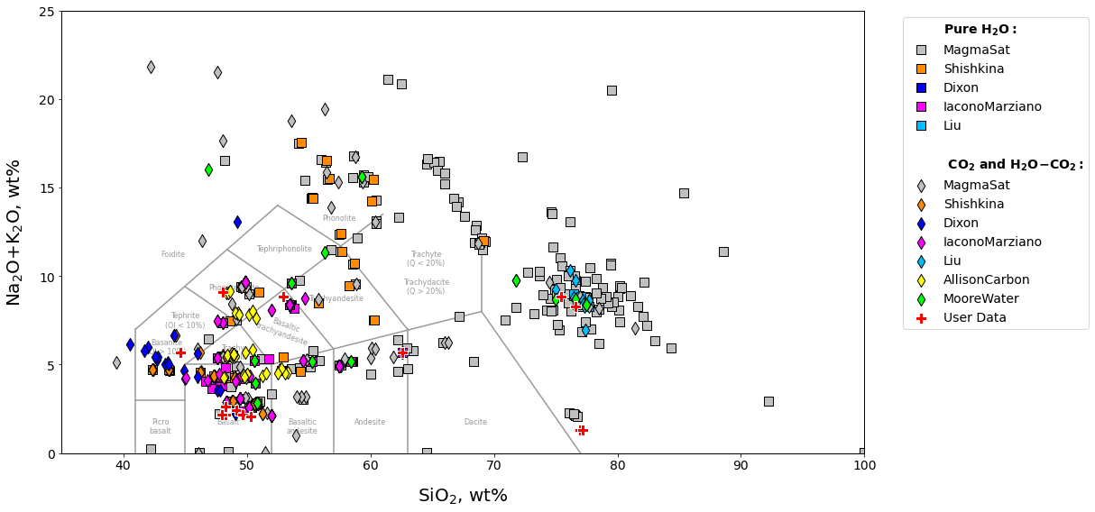
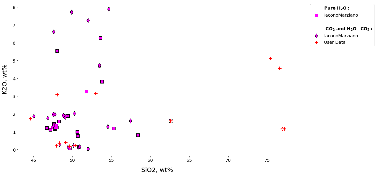
Figure 5:Example calibration plots. a. The default plot with user_data defined as myfile and no other options set. This produces a TAS diagram with the user data plotted atop data from calibration datasets for all models. b. A plot with all options specified. This example produces an x-y plot for user_data (myfile) and the Iacono-Marziano calibration dataset where x and y are SiO2 and K2O concentration in wt%. Symbol shapes correspond to the volatile composition of experiments used to calibrate the model.
Using the functionality built into python and the matplotlib library, user data can be plotted on its own at any time, including before any calculations are performed. Almost any plot type imaginable can be produced, and users should refer to the maptlotlib documentation (https://
3.5Calculating dissolved volatile concentrations
The calculate_dissolved_volatiles() function calculates the concentration of dissolved H2O and CO2 in the melt at a given pressure-temperature condition and with a given H2O-CO2 fluid composition, defined as the mole fraction of H2O in an H2O-CO2 fluid (XH2Ofluid). The default MagmaSat model relies on the underlying functionality of MELTS, whose basic function is to calculate the equilibrium phase assemblage given the bulk composition of the system and pressure-temperature conditions. To calculate dissolved volatile concentrations thus requires computing the equilibrium state of a system at fixed pressure and temperature over a range of bulk volatile concentrations until a solution is found that satisfies the user defined fluid composition.
First, the function makes an initial guess at the appropriate bulk volatile concentrations by finding the minimum dissolved volatile concentrations in the melt at saturation, while asserting that the weight fraction of H2O/(H2O+CO2) in the system is equal to the user input mole fraction of H2O/(H2O+CO2) in the fluid. This is done by increasing the H2O and CO2 concentrations appropriately until a fluid phase is stable. Once fluid saturation is determined, the code then performs directional, iterative, and progressively more refined searches, increasing the proportion of H2O or CO2 in the system if the mole fraction of H2O calculated in the fluid is greater than or less than that defined by the user, respectively. Four iterative searches are performed; the precision of the match between the calculated and defined XH2Ofluid increases from 0.1 in the first iteration to 0.01, 0.001, and finally to 0.0001. Thus, the calculated dissolved volatile concentrations correspond to a system with XH2Ofluid within 0.0001 of the user defined value.
For non-MagmaSat models, dissolved volatile concentrations are calculated directly from model equations.
- Method structure
Single sample:
calculate_dissolved_volatiles(sample, temperature, pressure, X_fluid=1, verbose=False, model='MagmaSat').resultBatchFile batch process:
myfile.calculate_dissolved_volatiles(temperature, pressure, X_fluid=1, print_status=True, model='MagmaSat')- Standard inputs
sample,temperature,pressure,X_fluid,model(see Section 3.1).- Unique optional inputs
verbose: Only for single sample calculations. Default value is False, in which case H2O and CO2 concentrations are returned. If set to True, additional parameters are returned in a dictionary: H2O and CO2 concentrations in the fluid in mole fraction, temperature, pressure, and proportion of the fluid in the system in wt%.print_status: Only for batch calculations. The default value is True, in which case the progress of the calculation will be printed to the terminal. The user may desire to see the status of the calculation, as this particular function can be quite slow, averaging between 3-5 seconds per sample.- Calculated outputs
If the single-sample method is used, a dictionary with keys ‘H2O’ and ‘CO2’ corresponding to the calculated dissolved H2O and CO2 concentrations in the melt is returned (plus additional variables ‘temperature’ in °C, ‘pressure’ in bars, ‘XH2O_fl’, ‘XCO2_fl’, and ‘FluidProportion_wtper’ (the proportion of the fluid in the system in wt%) if
verboseis set to True).If the BatchFile method is used, a pandas DataFrame is returned with sample information plus calculated dissolved H2O and CO2 concentrations in the melt, the fluid composition in mole fraction, and the proportion of the fluid in the system in wt%. Pressure (in bars) and Temperature (in °C) columns are always returned.
"""Calculate dissolved volatiles for sample 10*"""
v.calculate_dissolved_volatiles(sample=sample_10, temperature=900.0, pressure=2000.0,
                                X_fluid=0.5, verbose=True).result
{'H2O_liq': 2.69352739399806,
'CO2_liq': 0.0638439414375309,
'XH2O_fl': 0.500092686493868,
'XCO2_fl': 0.499907313506132,
'FluidProportion_wt': 0.18407321260435108}"""Calculate dissolved for all samples in an BatchFile object"""
dissolved = myfile.calculate_dissolved_volatiles(temperature=900.0, pressure=2000.0, X_fluid=1, print_status=True)Table 5:Modeled dissolved volatile concentrations
dissolved3.6Calculating equilibrium fluid compositions
The calculate_equilibrium_fluid_comp() function calculates the composition of a fluid phase in equilibrium with a given silicate melt with known pressure, temperature, and dissolved H2O and CO2 concentrations. The calculation is performed simply by calculating the equilibrium state of the given sample at the given conditions and determining if that melt is fluid saturated. If the melt is saturated, fluid composition and mass are reported back. If the calculation finds that the melt is not saturated at the given pressure and temperature, values of 0.0 will be returned for the H2O and CO2 concentrations in the fluid.
- Method structure
Single sample:
calculate_equilibrium_fluid_comp(sample, temperature, pressure, verbose=False, model='MagmaSat').resultBatchFile batch process:
myfile.calculate_equilibrium_fluid_comp(temperature, pressure=None, print_status=False, model='MagmaSat')- Standard inputs
sample,temperature,pressure,model(see Section 3.1).- Unique optional inputs
verbose: Only for single sample calculations. Default value is False, in which case H2O and CO2 concentrations in the fluid in mol fraction are returned. If set to True, additional parameters are returned in a dictionary: H2O and CO2 concentrations in the fluid, mass of the fluid in grams, and proportion of the fluid in the system in wt%.print_status: Only for batch calculations. The default value is False. If True is passed, the progress of the calculation will be printed to the terminal.- Calculated outputs
If the single-sample method is used, a dictionary with keys ‘H2O’ and ‘CO2’ is returned (plus additional variables ‘FluidMass_grams’ and ‘FluidProportion_wtper’ if
verboseis set to True).If the BatchFile method is used, a pandas DataFrame is returned with sample information plus calculated equilibrium fluid compositions, mass of the fluid in grams, and proportion of the fluid in the system in wt%. Pressure (in bars) and Temperature (in °C) columns are always returned.
"""Calculate fluid composition for the extracted sample"""
v.calculate_equilibrium_fluid_comp(sample=sample_10, temperature=900.0, pressure=100.0).result
{'CO2': 0.00528661429366132, 'H2O': 0.994713385706339}Below we calculate equilibrium fluid compositions for all samples at a single temperature of 900 °C and a single pressure of 1,000 bars. Note that some samples in this dataset have quite low volatile concentrations (e.g., the Tucker et al. (2019) basalts from Kilauea), and so are below saturation at this P-T condition. The fluid composition for undersaturated samples is returned as values of 0 for both H2O and CO2.
Table 6:Isothermally modeled equilibrium fluid compositions
"""Calculate fluid composition for all samples in an BatchFile object"""
eqfluid = myfile.calculate_equilibrium_fluid_comp(temperature=900.0, pressure=1000.0)
eqfluidBelow, we calculate equilibrium fluid compositions for the same dataset using temperatures and pressures as defined in the input data (Table 3). Note that Samples “samp. HPR3-1_XL-3” and “samp. HPR3-1_XL-4_INCL-1” have a user-defined value of 0.0 for temperature and pressure, respectively. VESIcal automatically skips the calculation of equilibrium fluids for these samples and returns a warning to the user, which are both printed to the terminal below and appended to the “Warnings” column in the returned data.
Table 7:Modeled equilibrium fluid compositions with unique temperatures. Warnings “Bad temperature” and “Bad pressure” indicate that no data (or 0.0 value data) was given for the temperature or pressure of that sample, in which case the calculation of that sample is skipped.
"""Calculate fluid composition for all samples with unique pressure and temperature values for each sample.
Pressure and temperature values are taken from columns named "Press" and "Temp" in the example BatchFile"""

eqfluid_wtemps = myfile.calculate_equilibrium_fluid_comp(temperature='Temp', pressure='Press')
eqfluid_wtemps3.6.1Converting fluid composition units
The fluid composition is always returned in units of mol fraction. Two functions exist to transform only the H2O-CO2 fluid composition between mol fraction and wt% and can be applied to returned data sets from calculations. Both functions require that the user provide the dataframe containing fluid composition information plus the names of the columns corresponding to the H2O and CO2 concentrations in the fluid. The default values for column names are set to those that may be returned by VESIcal core calculations, such that they need not be specified unless the user has changed them or is supplying their own data (e.g., imported data not processed through a core calculation).
- Method structure
Mol fraction to wt%:
fluid_molfrac_to_wt(data, H2O_colname='XH2O_fl_VESIcal', CO2_colname='XCO2_fl_VESIcal')Wt% to mol fraction:
fluid_wt_to_molfrac(data, H2O_colname='H2O_fl_wt', CO2_colname='CO2_fl_wt')- Required inputs
data: A pandas DataFrame containing columns for H2O and CO2 concentrations in the fluid.- Optional inputs
H2O_colnameandCO2_colname: The default values are ‘XH2O_fl’ and ‘XCO2_fl’ if input data are in mol fraction or ‘H2O_fl_wt’ and ‘CO2_fl_wt’ if the data are in wt%. Strings containing the name of the columns corresponding to the H2O and CO2 concentrations in the fluid.- Calculated outputs
The original data passed plus newly calculated values are returned in a DataFrame.
Table 8:Equilibrium fluid compositions converted from mol fraction to wt%
"""Converting from mol fraction to wt%"""
eqfluid_wt = v.fluid_molfrac_to_wt(eqfluid)
eqfluid_wtTable 9:Equilibrium fluid compositions converted from wt% to mol fraction
"""Converting from wt% to mol fraction"""
eqfluid_mol = v.fluid_wt_to_molfrac(eqfluid_wt)
eqfluid_mol3.7Calculating saturation pressures
The calculate_saturation_pressure() function calculates the minimum pressure at which a given silicate melt with known temperature and H2O and CO2 concentrations would be saturated with fluid. For MagmaSat, this is calculated by finding the pressure at which the smallest amount of vapor is present. This function also calculates the composition of the vapor in equilibrium with the melt at those conditions.
The function works by calculating the equilibrium state of the given melt at very high pressure (20,000 bars). If no fluid is present at this pressure, the melt is undersaturated, and pressure is decreased in steps of 1,000 bars until the mass of vapor is >0 grams. If fluid is present, the saturation limit is found by increasing the pressure iteratively until the point at which no fluid is present. At this point, the pressure space is narrowed and searched in steps of 100 bars and then in steps of 10 bars until the saturation pressure is found. Thus, these calculations are accurate to 10 bars.
For non-MagmaSat models, we use Brent’s minimization method (via scipy’s root_scalar optimization function) to find the pressure that satisfies the computational constraints. This is achieved by iterative calculation of the dissolved volatile concentration over a range of pressures and minimizing the difference between computed and given concentrations. This is only practical for non-MagmaSat models, where the dissolved volatiles calculation is extremely fast.
- Method structure
Single sample:
calculate_saturation_pressure(sample, temperature, verbose=False, model='MagmaSat').resultBatchFile batch process:
myfile.calculate_saturation_pressure(temperature, print_status=True, model='MagmaSat')- Standard inputs
sample,temperature,model(see Section 3.1).- Unique optional inputs
verbose: Only for single sample calculations. Default value is False, in which case the saturation pressure in bars is returned. If set to True, additional parameters are returned in a dictionary: saturation pressure in bars, H2O and CO2 concentrations in the fluid, mass of the fluid in grams, and proportion of the fluid in the system in wt%.print_status: Only for batch calculations. The default value is True, in which case the progress of the calculation will be printed to the terminal.- Calculated outputs
If the single-sample method is used, the saturation pressure in bars is returned as a numerical value (float) (plus additional variables ‘XH2O_fl’, ‘XCO2_fl’, ‘FluidMass_grams’, and ‘FluidProportion_wtper’ if
verboseis set to True).If the BatchFile method is used, a pandas DataFrame is returned with sample information plus calculated saturation pressures, equilibrium fluid compositions, mass of the fluid in grams, and proportion of the fluid in the system in wt%. Temperature (in °C) is always returned.
"""Calculate the saturation pressure of the single sample we defined in Section 3.3.1 at 925 degrees C"""
v.calculate_saturation_pressure(sample=mysample, temperature=925.0, verbose=True).result
{'SaturationP_bars': 2960,
'FluidMass_grams': 0.0018160337487088,
'FluidProportion_wt': 0.0018160337487087978,
'XH2O_fl': 0.838064480487942,
'XCO2_fl': 0.161935519512058}Table 10:Isothermally modeled saturation pressures
"""Calculate the saturation pressure for all samples in an BatchFile object at 925 degrees C"""
satPs = myfile.calculate_saturation_pressure(temperature=925.0)
satPsTable 11:Modeled saturation pressures with unique temperatures The warning “Bad temperature” indicates that no data (or 0.0 value data) was given for the temperature of that sample, in which case the calculation of that sample is skipped.
"""Calculate the saturation pressure for all samples in an BatchFile object, taking temperature
values from a column named "Temp" in the BatchFile"""
satPs_wtemps = myfile.calculate_saturation_pressure(temperature="Temp")
satPs_wtemps3.8Calculating isobars and isopleths
In this example, we demonstrate how isobars (lines of constant pressure) and isopleths (lines of constant fluid composition) can be calculated for any one composition. A single melt composition can be extracted from a loaded batch file, or a composition can be entered by hand and stored within a dictionary. Due to computational intensity, isobars and isopleths can only be computed for one sample composition at a time.
Once a single composition is defined, conditions over which to calculate isobars and isopleths must be specified. The generated plot is isothermal, so only one temperature can be chosen. Isobars and isopleths can be calculated for any number of pressures or XH2Ofluid values, respectively, passed as lists.
The calculation is performed by iterating through possible concentrations of H2O and CO2 and calculating the equilibrium state for the system. The iteration begins at a fixed H2O concentration, increasing the CO2 concentration in steps of 0.1 wt% until a fluid phase is stable. The H2O concentration is then increased by 0.5 wt% and CO2 is again increased from 0 until a fluid phase is stable. This process is repeated for H2O values ranging from 0–15 wt%. The H2O and CO2 concentrations from each system for which a fluid phase was found to be stable are saved and written to a pandas DataFrame, which is returned upon completion of the calculation.
Isobars and isopleths are computed at fixed H2O-CO2 points for any given pressure. To generate curves using the MagmaSat model, polynomials are fit to computed points using numpy’s polyfit method. This can be optionally disabled by setting smooth_isobars or smooth_isopleths to False. The curvature of the isobars depends strongly on the number of points used to fit a polynomial, deemed “control points”, with curve fits becoming more accurate to the model as the number of control points increases. We found that above five control points, changes to the shape of the curve fits becomes negligible. Thus, as a compromise between accuracy and computation time, and to maintain consistency, MagmaSat isobars are always computed with 5 control points at XH2Ofluid values of 0, 0.25, 0.5, 0.75, and 1. Because non-MagmaSat models compute extremely quickly, all non-MagmaSat models use 51 control points per isobar and do not utilize polynomial fits to the data by default.
- Method structure
Only single sample calculations.
calculate_isobars_and_isopleths(sample, temperature, pressure_list, isopleth_list=None, smooth_isobars=True, smooth_isopleths=True, print_status=True, model="MagmaSat").result- Standard inputs
sample,temperature,model(see Section 3.1).- Unique required inputs
pressure_list: A list of all pressures in bars at which to calculate isobars. If only one value is passed it can be as float instead of list.- Unique optional inputs
isopleth_list: The default value is None in which case only isobars will be calculated. A list of all fluid composition values, in mole fraction H2O (XH2Ofluid), at which to calculate isopleths. Values can range from 0–1. If only one value is passed it can be as float instead of list. N.b. that, due to the method of isobar smoothing using control points as outlined above, each isopleth value passed here not equal to one of the five standard control point values (0, 0.25, 0.5, 0.75, or 1) will result in an an additional control point being used to smooth the isobars. Thus, entering additional isopleth values results not only in more isopleth outputs but also in “smoother” (i.e., more well constrained) isobars.smooth_isobarsandsmooth_isopleths: The default value for both of these arguments is True, in which case polynomials will be fit to the computed data points.print_status: The default value is True. If True, the progress of the calculations will be printed to the terminal.- Calculated outputs
The function returns two pandas DataFrames: the first has isobar data, and the second has isopleth data. Columns in the isobar dataframe are ‘Pressure’, ‘H2Omelt’, and ‘CO2melt’, corresponding to pressure in bars and dissolved H2O and CO2 in the melt in wt%. Columns in the isopleth dataframe are ‘XH2O_fl’, ‘H2O_liq’, and ‘CO2_liq’, corresponding to XH2Ofluid and dissolved H2O and CO2 in the melt in wt%.
"""Define all variables to be passed to the function for calculating isobars and isopleths"""
"""Define the temperature in degrees C"""
temperature = 1200.0

"""Define a list of pressures in bars:"""
pressures = [1000.0, 2000.0, 3000.0]
Next, the H2O and CO2 dissolved in the melt at saturation is calculated at the specified temperature and over the range of specified pressures. Note that, because this function calculates two things (isobars and isopleths), two variable names must be given (below, “isobars, isopleths”). This calculation can be quite slow, and so it is recommended to set print_status to True.
isobars, isopleths = v.calculate_isobars_and_isopleths(sample=sample_10,
                                            temperature=temperature,
                                            pressure_list=pressures,
                                            isopleth_list=[0.25,0.5,0.75]).result
Calculating isobar at 1000.0 bars
done.
Calculating isobar at 2000.0 bars
done.
Calculating isobar at 3000.0 bars
done.
Done!
3.9Calculating degassing paths
A degassing path is a series of volatile concentrations both in the melt and fluid that a magma will follow during decompression. In the calculation, the saturation pressure is computed, and then the system is equilibrated along a trajectory of decreasing pressure values at discrete steps. The default number of steps to calculate is 50, but this can be defined by the user by setting the argument steps to any integer value. A detailed explanation of how non-MagmaSat models handle the calculation of mixed-fluid composition can be found in the supplement (Supplementary Text S2). If so desired, this calculation can be performed for any initial pressure, but the default is the saturation pressure. If a pressure is specified that is above the saturation pressure, the calculation will simply proceed from the saturation pressure, since the magma cannot degas until it reaches saturation.
Completely open-system, completely closed-system or partially open-system degassing paths can be calculated by specifying what proportion of the fluid to fractionate. The fluid fractionation value can range between 0 (closed-system: no fluid is removed, all is retained at each pressure step) and 1 (open-system: all fluid is removed, none is retained at each pressure step). Closed and partially open-system runs allow the user to specify the initial presence of exsolved fluid that is in equilibrium with the melt at the starting pressure.
- Method structure
Only single-sample calculations.
calculate_degassing_path(sample, temperature, pressure="saturation", fractionate_vapor=0.0, init_vapor=0.0, steps=50, model="MagmaSat").result- Standard inputs
sample,temperature,model(see Section 3.1).- Unique optional inputs
pressure: The pressure at which to begin the degassing calculations, in bars. Default value is ‘saturation’, which runs the calculation with the initial pressure at the saturation pressure. If a pressure greater than the saturation pressure is input, the calculation will start at saturation, since this is the first pressure at which any degassing will occur.fractionate_vapor: Proportion of vapor removed at each pressure step. Default value is 0.0 (completely closed-system degassing). Specifies the type of calculation performed, either closed system (0.0) or open system (1.0) degassing. If any value between <1.0 is chosen, user can also specify the ‘init_vapor’ argument (see below). A value in between 0 and 1 will remove that proportion of vapor at each step. For example, for a value of 0.2, the calculation will remove 20% of the vapor and retain 80% of the vapor at each pressure step.init_vapor: Default value is 0.0. Specifies the amount of vapor (in wt%) coexisting with the melt before degassing.steps: Default value is 50. Specifies the number of steps in pressure space at which to calculate dissolved volatile concentrations.- Calculated outputs
The function returns a pandas DataFrame with columns as: ‘Pressure_bars’, ‘H2O_liq’ and ‘CO2_liq’ (the concentration of H2O and CO2 in the melt, in wt%), ‘XH2O_fl’ and ‘XCO2_fl’ (the composition of the H2O-CO2 fluid, in mol fraction), and ‘FluidProportion_wt’ (the proportion of fluid in the fluid-melt system, in wt%).
Note: The following two cells can take up to a minute to execute.
temp = 1200 #temperature in °C

"""Calculate open, closed, and closed + 2 wt% initial vapor"""
closed_df = v.calculate_degassing_path(sample=sample_10, temperature=temp).result
open_df = v.calculate_degassing_path(sample=sample_10, temperature=temp, fractionate_vapor=1.0).result
half_df = v.calculate_degassing_path(sample=sample_10, temperature=temp, fractionate_vapor=0.5).result
exsolved_df = v.calculate_degassing_path(sample=sample_10, temperature=temp, init_vapor=2.0).result
"""Calculate closed-system degassing starting from a pressure of 2000 bars"""
start2000_df = v.calculate_degassing_path(sample=sample_10, temperature=temp, pressure=2000.0).result3.10Plotting
After calculating isobars, isopleths, and degassing paths, any or all of these may be plotted in an H2O versus CO2 plot with one simple function call. The plot will be printed directly in the notebook or, if the code is run as script in a command line, the plot will appear it its own window, at which point it can be saved as an image file. VESIcal’s plot function takes in lists of pandas DataFrames with calculated isobar, isopleth, and degassing path information (e.g., output from calculate_isobars_and_isopleths() or calculate_degassing_path()) and plots data as isobars (lines of constant pressure), isopleths (lines of constant fluid composition), and degassing paths (lines indicating the concentrations of H2O and CO2 in a melt equilibrated along a path of decreasing pressure).
Labels can be assigned to isobars, isopleths, and/or degassing paths separately. Any or all of these data can be passed to the plot function. Multiple sets of plottable data can be passed. For example, isobars calculated with two different models can be passed to the isobars argument as a list.
VESIcal’s plotting function is entirely based on python’s matplotlib library, which comes standard with many installations of python. With matplotlib, users can create a large variety of plots (note that direct matplotlib functionality is used to create custom plots in several of this manuscript’s supplementary Jupyter notebooks), and users should refer to the maptlotlib documentation (https://
The function returns both fig and axes matplotlib objects, which can be further edited by the user or plotted directly. Following matplotlib convention, the results of plot() should be saved to objects such as fig, ax as:
fig, ax = v.plot([options])
where [options] represents any optional inputs as defined here. Variables fig and ax can then be edited further using matplotlib tools. For example, the user might wish to set the minimum x-axis value to 0.5 as:
ax.set_xlim(left=0.5)
In Jupyter Notebook, a plot is automatically shown, but in the command line, the plot will only display after executing v.show().
- Method structure
plot(isobars=None, isopleths=None, degassing_paths=None, custom_H2O=None, custom_CO2=None, isobar_labels=None, isopleth_labels=None, degassing_path_labels=None, custom_labels=None, custom_colors="VESIcal", custom_symbols=None, markersize=10, save_fig=False, extend_isobars_to_zero=True, smooth_isobars=False, smooth_isopleths=False)- Optional inputs
isobars: DataFrame object containing isobar information as calculated bycalculate_isobars_and_isopleths(). Or a list of DataFrame objects.isopleths: DataFrame object containing isopleth information as calculated bycalculate_isobars_and_isopleths(). Or a list of DataFrame objects.degassing_paths: List of DataFrames with degassing information as generated bycalculate_degassing_path().custom_H2O: List of floats or array-like shapes of H2O concentration values to plot as points. For examplemyfile.data['H2O']is one array-like shape (here, pandas.Series) of H2O values. Must be passed withcustom_CO2and must be same length ascustom_CO2.custom_CO2: List of floats or array-like shapes of CO2 values to plot as points. For examplemyfile.data['CO2']is one array-like shape of CO2 values. Must be passed withcustom_H2Oand must be same length ascustom_H2O.isobar_labels: Labels for the plot legend. Default is None, in which case each plotted line will be given the generic legend name of “Isobars n”, with n referring to the nth isobars passed. Isobar pressure is given in parentheses. The user can pass their own labels as a list of strings. If more than one set of isobars is passed, the labels should refer to each set of isobars, not each pressure.isopleth_labels: Labels for the plot legend. Default is None, in which case each plotted isopleth will be given the generic legend name of “Isopleth n”, with n referring to the nth isopleths passed. Isopleth XH2O values are given in parentheses. The user can pass their own labels as a list of strings. If more than one set of isopleths is passed, the labels should refer to each set of isopleths, not each XH2O value.degassing_path_labels: Labels for the plot legend. Default is None, in which case each plotted line will be given the generic legend name of “Pathn”, with n referring to the nth degassing path passed. The user can pass their own labels as a list of strings.custom_labels: Labels for the plot legend. Default is None, in which case each group of custom points will be given the generic legend name of “Customn”, with n referring to the nth degassing path passed. The user can pass their own labels as a list of strings.custom_colorsandcustom_symbols: Custom colors and symbol shapes can be specified for (custom_H2O,custom_CO2) points. A list of color values or symbol types readable by Matplotlib (see Matplotlib documentation) can be entered. The length of this list must be equal to the lengths ofcustom_H2Oandcustom_CO2. If nothing is specified for custom_colors, VESIcal’s default colors will be used. If nothing is specified forcustom_symbols, all points will be plotted as filled circles.markersize: The size of the symbols can be specified here. If not specified, the default value is marker size 10.save_fig: Default value is False, in which case the figure will not be saved. If a string is passed, the figure will be saved with the string as the filename. The string must include the file extension.- Advanced inputs: Most users will not need to use these inputs.
extend_isobars_to_zero: If set to True (the default), isobars will be extended to the plot axes, which are at x=0 and y=0, even if there is a finite solubility at zero partial pressure.smooth_isobarsandsmooth_isopleths: If set to True, isobar or isopleth data will be fit to a polynomial and plotted. If set to False (the default), the raw input data will be plotted. Note that MagmaSatcalculate_isobars_and_isopleths()calculations return already “smoothed” data (that is, the raw data are fit to polynomials before being returned). Raw “unsmoothed” data can be returned by MagmaSatcalculate_isobars_and_isopleths()(see documentation on this method).- Calculated outputs
The function returns fig and axes matplotlib objects defining a plot with x-axis as H2O wt% in the melt and y-axis as CO2 wt% in the melt. Isobars, or lines of constant pressure at which the sample magma composition is saturated, and isopleths, or lines of constant fluid composition at which the sample magma composition is saturated, are plotted if passed. Degassing paths, or the concentration of dissolved H2O and CO2 in a melt equilibrated along a path of decreasing pressure, is plotted if passed.
3.10.1A simple example: Isobars and isopleths
Here we plot the isobars at 1,000, 2,000, and 3,000 bars and isopleths at 0.25, 0.5, and 0.75 XH2Ofluid calculated for sample ‘10*’ at 1,200 °C in Section 3.8 onto one plot.
fig, ax = v.plot(isobars=isobars, isopleths=isopleths)
v.show()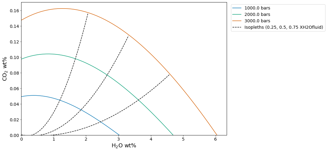
Figure 6:Isobars and isopleths calculated for the sample, temperature, pressures, XH2Ofluid values, and with the model as defined in Section 3.8. Manuscript default values are sample 10* at a 1,200 °C with isobars at 1,000, 2,000, and 3,000 bars, isopleths at XH2Ofluid = 0, 0.25, 0.5, 0.75, and 1 calculated with MagmaSat
When plotting isobars and isopleths via MagmaSat, the values calculated by calculate_isobars_and_isopleths() are used to calculate polynomial fits using Numpy’s polyfit. These polynomial fits, not the raw calculated data, are what have been plotted above. This method of fitting polynomial curves to these data is common in the literature e.g., Newman & Lowenstern, 2002Iacono-Marziano et al., 2012Iacovino et al., 2013 and is likely a very close approximation of the true saturation surface. Non-MagmaSat models do not calculate polynomial fits by default, but this can be done by passing smooth_isobars=True and smooth_isopleths=True to plot().
A user may wish to apply custom formatting to the plot, in which case the polynomial fits can be calculated and returned as a pandas DataFrame, which the user can then plot up manually using Matplotlib, MS Excel, or some other preferred method. To calculate polynomial fits to isobar and isopleth data, isobars and isopleths can be passed to smooth_isobars_and_isopleths(). For this advanced case, we refer the reader to the documentation.
3.10.2A simple example: Degassing paths
Here we plot all four degassing paths calculated for sample ‘10*’ at 1,200 °C in Section 3.9 onto one plot. We designate labels of “Open”, “Half”, “Closed”, and “Exsolved” for the legend.
fig, ax = v.plot(degassing_paths=[open_df, half_df, closed_df, exsolved_df],
            degassing_path_labels=["Open", "Half", "Closed", "Exsolved"])
fig, ax = v.plot(degassing_paths=[exsolved_df, start2000_df],
            degassing_path_labels=["Exsolved", "2000 bars"])
v.show()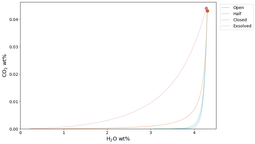
Figure 7:Degassing paths calculated for the sample, temperature, degassing style, initial exsolved fluid wt%, starting pressure, and model as designated in Section 3.9. Default manuscript values are sample 10* at 1,200 °C. “Open”, “Half”, and “Closed” curves in (a) represent open-system, partially open-system (50% fractionated fluid), and closed-system degassing paths, respectively, starting at the saturation pressure. The “Exsolved” curve in (b) represents closed-system degassing with an initial exsolved fluid wt% = 2.0. The “2000” curve in (b) represents closed-system degassing calculated starting at a pressure of 2,000 bars.
3.10.3Plotting multiple calculations
One of the major advantages to VESIcal over any other modeling tool is the ability to quickly calculate and plot multiple calculations. VESIcal’s plot() function is built on top of the popular Matplotlib python library and is designed to work with any VESIcal generated data. It can automatically plot and label one or multiple calculations. In addition, it can plot, as a scatter plot, any x-y points. The plot function always generates plots with H2O on the x-axis and CO2 on the y-axis. scatterplot() will take in and plot any x-y data with custom x- and y-axis labels. Generating other commonly used petrologic plots (e.g. Harker style diagrams) is already possible with Matplotlib, and so VESIcal does not duplicate this functionality, however this may be added in future updates.
It may be tempting to plot multiple calculations on multiple samples and compare them, however we strongly caution against plotting data that do not correspond. For example, isobars and isopleths are calculated isothermally. If degassing paths are also plotted, the user should ensure that the degassing paths were calculated at the same temperature as the isobars and isopleths.
3.10.3.1Isobars, isopleths, and degassing paths
In this example we will use data imported in Section 3.4 and calculations performed in Sections 3.7 and 3.8. Of course, all of the data calculated with VESIcal can be exported to an Excel or CSV file for manipulation and plotting as desired. However, some examples of plotting that can be done within this notebook or in a python script are shown below. Here we plot:
- Isobars calculated at 1200 °C and pressures of 1,000, 2,000, and 3,000 bars for sample 10*
- Isopleths calculated at 1200 °C and XH2Ofluid values of 0, 0.25, 0.5, 0.75, and 1 for sample 10*
- An open-system degassing path for sample 10*
- A closed-system degassing path for sample 10*
fig, ax = v.plot(isobars=isobars,
                   isopleths=isopleths,
                   degassing_paths=[open_df, closed_df],
                   degassing_path_labels=["Open System", "Closed System"])
v.show()
Figure 8:Example of plotting multiple calculations on one plot. Isobars and isopleths as defined in Section 3.8 and shown in Section 3.10.1 and degassing curves as defined in Section 3.9 and shown in Section 3.10.2. Default manuscript values are for sample 10* at 1,200 °C with isobars at 1,000, 2,000, and 3,000 bars, isopleths at XH2Ofluid values of 0, 0.25, 0.5, 0.75, and 1 with an open-system and a closed-system degassing path.
3.10.3.2Isobars, isopleths, and degassing paths for multiple samples
First, we will calculate some new data for two different samples: a basanite sample KI-07 from Iacovino et al., 2016 and a rhyolite sample samp. P1968a from Myers et al., 2019. For both samples we will calculate and then plot:
- Isobars and isopleths at 1100 °C, pressures of 1,000 and 2,000 bars and fluid compositions of XH2Ofluid of 0.25, 0.5, and 0.75
- Closed-system degassing paths at 1100 °C
basanite_sample = myfile.get_sample_composition('KI-07', asSampleClass=True)
rhyolite_sample = myfile.get_sample_composition('samp. P1968a', asSampleClass=True)

basanite_isobars, basanite_isopleths = v.calculate_isobars_and_isopleths(sample=basanite_sample,
                                                                         temperature=1100,
                                                                         pressure_list=[1000, 2000],
                                                                         isopleth_list=[0.25,0.75]).result

rhyolite_isobars, rhyolite_isopleths = v.calculate_isobars_and_isopleths(sample=rhyolite_sample,
                                                                         temperature=1100,
                                                                         pressure_list=[1000, 2000],
                                                                         isopleth_list=[0.25,0.75]).result

basanite_degassing_path = v.calculate_degassing_path(sample=basanite_sample,
                                                     temperature=1100).result

rhyolite_degassing_path = v.calculate_degassing_path(sample=rhyolite_sample,
temperature=1100).resultfig, ax = v.plot(isobars=[basanite_isobars, rhyolite_isobars],
isopleths=[basanite_isopleths, rhyolite_isopleths],
degassing_paths=[basanite_degassing_path, rhyolite_degassing_path],
isobar_labels=["Basanite", "Rhyolite"],
isopleth_labels=["Basanite", "Rhyolite"],
degassing_path_labels=["Basanite", "Rhyolite"])
v.show()
Figure 9:Example of plotting multiple calculations from multiple samples on the same plot. Note that the colors are automatically set to correspond to each sample for all plotted items (here, isobars, isopleths, and degassing paths). Samples, pressures, temperatures, XH2Ofluid values, and degassing path styles are defined above in this section. Manuscript default values are for a basanite (sample KI-07) and a rhyolite (sample samp. P1968a) at 1,100 °C, 1,000 and 2,000 bars, and XH2Ofluid = 0.25 and 0.75 and closed-system degassing.
3.11Model hybridization (Advanced)
One of the advantages of implementing the solubility models in a generic python module is the flexibility this affords the user in changing the way solubility models are defined and used. In particular, the structure allows any combination of pure-fluid models to be used together in modeling mixed-fluids, and fugacity or activity models can be quickly changed without modifying code. This allows advanced users to see how changing a fugacity or activity model implemented in any particular solubility model would affect model results. Instructions for hybridizing models can be found in Supplemental Jupyter notebook S10.
3.12Exporting data
Once batch calculations have been performed, they can be exported to an Excel or CSV file with the save_excel() and save_csv() commands. These operations require that the user define a filename (what to name your new file) and a list of the calculation results to save to this file or files.
Note that this requires that calculations have been assigned to variable names, which has been done in all of the given examples. For example, to calculate saturation pressures of an imported file saved to the variable ‘myfile’ and simply print the output, the user can type myfile.calculate_saturation_pressures([options]), where ‘[options]’ are the required and optional inputs. However, to save this result to a variable (e.g., called ‘my_satPs’) so that it can be accessed later, the correct python syntax would be my_satPs = myfile.calculate_saturation_pressures([options]).
Multiple calculations can be saved at once. If saving to an Excel file, each calculation is saved as its own sheet within a single file. If desired, the user can define the names of each of these sheets. If not specified, the sheets will be named ‘Original_User_Data’, which contains the original input data, and then ‘CalcN’ where N is the nth calculation in a list of calculations. If saving multiple calculations to a CSV file, each calculation will be saved to its own CSV file, and a file name for each of these is required.
Advanced users note that the calculations argument takes in any pandas DataFrame object, meaning this functionality is not limited to VESIcal’s prescribed outputs. The save_excel() and save_csv() methods use the pandas to_excel and to_csv methods, however not all options are implemented here. If saving to a CSV file, any arguments that can be passed to pandas to_csv method may be passed to VESIcal’s save_csv().
- Method structures
save_excel(filename, calculations, sheet_name=None)save_csv(filenames, calculations)save_excel()Required inputsfilename(Excel): Name of the file to create. The extension (.xlsx) should be included along with the name itself, all in quotes (e.g.,filename='myfile.xlsx').calculations: A list of variables containing calculated outputs from any of the core BatchFile functions:calculate_dissolved_volatiles(),calculate_equilibrium_fluid_comp(), andcalculate_saturation_pressure(). This must be passed as a list type variable, even if only one calculation is given. This is done by enclosing the variable in square brackets (e.g.,calculations=[my_calculation]).save_excel()Optional inputssheet_name: The default value is None, in which case sheets will be saved as ‘Original_User_data’ (the data input by the user) followed by ‘CalcN’ where N is the nth calculation incalculations. Otherwise, a list of names for the sheets can be passed, with the names in quotes (e.g.sheet_name=['SaturationPressures']). ‘Original_User_data’ will always be saved as the first sheet.save_csv()Required inputsfilenames(CSV): Name of the file or files to create. The extension (.csv) should be included. If more than one filename is passed, it should be passed as a list. This is done by enclosing the filenames in square brackets (e.g.,filenames=["file1.csv", "file2.csv"]).calculations: same as forsave_excel(). Must be same length asfilenames.- Calculated outputs
- An Excel or CSV file or files will be saved to the active directory (i.e., the same folder as this manuscript notebook or wherever the code is being used).
Here we save five of the calculations performed on an imported data file earlier in this manuscript. The original user-input data are stored in the BatchFile object ‘myfile’. In the following line we use the method save_excel() to save the original data and a list of calculations given by the calculations argument to an Excel file.
myfile.save_excel(filename='testsave.xlsx',
                      calculations=[dissolved, eqfluid, eqfluid_wtemps, satPs, satPs_wtemps],
sheet_names=['dissolved', 'eqfluid', 'eqfluid_wtemps', 'SaturationPs', 'SatPs_wtemps'])3.12.1Saving data for re-import into VESIcal
In many cases, it may be preferable to compute large amounts of data using VESIcal and then reimport them, either to perform more analysis or to plot the data. Likewise, a user may wish to compute data in VESIcal and then send the results to a colleague, who can then re-import that data into VESIcal directly. For this case, we suggest using python’s pickle package (https://
Below we pickle our computed dissolved volatile concentrations by dumping our variable dissolved to a pickle file that we name “dissolved.p”.
import pickle

pickle.dump(dissolved, open("dissolved.p", "wb"))
In another python file or terminal session, dissolved can be loaded back in via:
import pickle

dissolved = pickle.load(open("dissolved.p", "rb"))4Discussion and Applications
4.1Compositional Variation Within Datasets and Best Practices
It has been clearly shown that the composition of a melt plays a strong role in determining the solubility of H2O and CO2 in magmas Papale et al., 2006Moore, 2008Ghiorso & Gualda, 2015Wieser et al., 2021. Thus, compositional variance must be accounted for in any study examining solubility in multiple samples. A key use case where VESIcal can facilitate the adoption of this practice is in melt inclusion (MI) studies; specifically, where a single suite of MI with multiple melt compositions is examined using solubility models to interrogate magmatic degassing processes. Prior to the availability of VESIcal, the difficulty associated with performing multiple model calculations on multiple samples resulted in very few studies accounting for any compositional variance within their datasets. Indeed, until now, it has been difficult to even assess whether the potentially minimal compositional variance within a suite of melt inclusions from a single volcanic eruption would have any measurable effect on solubilities calculated for different MI.
Using VESIcal, we can address the question: what is the quantitative effect of compositional variation within a single suite of melt inclusions upon calculated melt inclusion saturation pressures? And, how does this affect conclusions that might be drawn regarding volcanic degassing and eruptive processes? To investigate this, we use a dataset of basaltic melt inclusions from Cerro Negro volcano, Nicaragua Roggensack, 2001. The compositional variation of these MI Figure 10, while relatively restricted, results in quite variable mixed-fluid solubilities from sample to sample. To determine the end-member compositions within the dataset corresponding to the samples with the maximum and minimum combined H2O-CO2 solubilities, isobars were computed at 1200 °C and 3,000 bars for all samples using the MagmaSat model in VESIcal. Maximum and minimum samples were taken as the isobar curves with the smallest and largest integral (area under the curve). We refer to this value as the “integrated mixed-volatile solubility” value, IMS, in units of concentration squared. The samples that produced maximum and minimum integrated solubilities are shown in Figures 10 and 11 in blue and green, respectively (sample 41b*, IMS=0.81 and 36a*, IMS=0.66 wt%2 at 3,000 bars). A composition representing the average of all MI in the dataset is shown in orange (“Average Sample”, IMS=0.70 wt%2 at 3,000 bars). A Jupyter notebook to reproduce these calculations is provided in the supplement (Supplementary Jupyter Notebook S8).
Figure 10:Harker style diagrams illustrating the compositional range of MIs from Cerro Negro volcano from Roggensack (2001). The “Average Sample” plotted as an orange dot represents a fictitious sample, calculated as the average of all MIs in the dataset. Sample 41b* and 36a* are the names of samples that produced isobars with maximum and minimum area under the curve, respectively (see text). Gray diamonds are all other data in the dataset.

Figure 11:H2O-CO2 diagram with isobars for MI from Cerro Negro volcano Roggensack (2001) computed by VESIcal using MagmaSat at 1200 °C, pressures of 500, 1000, 2000, 3000, and 4,000 bars. Curves shown are polynomials fitted to data computed by VESIcal. Blue and green curves correspond to samples 41b* and 36a*, which produced isobars with maximum and minimum area under the curve, respectively. Orange isobars were those computed for a fictitious sample representing the average composition of the MI dataset. Gray diamonds are all other data in the dataset.
At all pressures, the integrated mixed-volatile solubility across the Cerro Negro dataset varies as much as 10% relative Figure 11. For these MI, this results in as much as 11.5% relative error in the calculation of saturation pressures (average error for the entire dataset of 6.8% relative). It is noteworthy that this error is not systematic either in terms of absolute value or sign. For example, when calculated using their own compositions, saturation pressures for maximum and minimum samples 41b* and 36a* are 3050 and 3090 bars, respectively. But, saturation pressures calculated for both of these MI using the dataset’s average composition are 3020 and 3250 bars, respectively. That is an error of -30 and +160 bars or -1% and +5% respectively. Errors in these calculations, thus, may be quite small. But, in any case, removing this error completely is a simple task using VESIcal, and so we recommend that studies adopt the practice of calculating volatile solubilities (and associated values) in melts using the composition unique to each melt investigated.
Even in cases where solubility values (e.g., saturation pressures) are not calculated, the error highlighted above plagues any isobar diagram over which multiple melt compositions are plotted (e.g., Figure 11). Alternative plots to the commonly used H2O-CO2 diagram are shown in Figure 12, in which the same dataset is plotted in terms of computed saturation pressure (at 1200 °C calculated with VESIcal using MagmaSat) versus dissolved H2O, dissolved CO2, and fluid composition (as XH2Ofluid calculated with VESIcal using MagmaSat). These plots avoid the issues discussed above as they are compositionally independent, since the saturation pressure is calculated individually for each sample composition. Degassing trends are more accurately represented; H2O and CO2 concentrations lie along expected degassing trends with much less scatter than the H2O-CO2 plot. We can also see from this figure that the fluid composition during this eruption at Cerro Negro remained relatively constant at XH2Ofluid 0.8 from reservoir to surface, suggesting a scenario approaching closed-system degassing (i.e., melt volatile concentrations are buffered by the co-existing fluid composition). This is discussed in more detail in the companion paper Wieser et al., 2021.

Figure 12:Saturation pressure at 1200 °C calculated using VESIcal with MagmaSat versus measured dissolved H2O and CO2 concentrations and calculated fluid composition in Cerro Negro melt inclusions. These plots meaningfully illustrate degassing processes while avoiding issues associated with commonly used H2O-CO2 diagrams, which occur with even minor compositional variation within a given dataset.
4.2Model Comparisons
One of the possible workflows enabled through VESIcal is the ability to compute and compare (numerically and graphically) results from several models at once. To illustrate this point, we will take two single samples within the calibrated compositional range of several models, calculate isobars at multiple pressures, and plot the results. This is a common way to compare the solubility surface computed by different models for a single melt composition, and it is particularly useful since it quickly highlights the significant variation that exists between published models. The results of this exercise are shown here, and a Jupyter notebook to reproduce the code and calibration checks is available in the Supplement (Supplementary Jupyter Notebook S9).
We use a fictitious alkali basalt that we name “alkbasalt” and a fictitious rhyolite whose compositions are given in Table 12. The use of VESIcal’s calib_plot() function (see supplement) illustrates that the composition of the alkali basalt is within the compositional calibration ranges of four mixed-fluid solubility models: MagmaSat, Iacono-Marziano, Dixon, and ShishkinaIdealMixing. The rhyolite is within the ranges of MagmaSat and Liu. Isobars were calculated with these models at 1200 °C for alkbasalt and 800 °C for rhyolite and pressures of 500, 1,000, and 2,000 bars, using the below code:
Table 12:Melt compositions used for modeling
model_comps = v.BatchFile("tables/Table_Model_Comps.xlsx")
model_comps.dataalkbasalt = model_comps.get_sample_composition("Alkali Basalt", asSampleClass=True)
rhyolite = model_comps.get_sample_composition("Rhyolite", asSampleClass=True)
alkbasalt_isobars, alkbasalt_isopleths = v.calculate_isobars_and_isopleths(sample=alkbasalt,
temperature=1200, pressure_list=[500, 1000, 2000],
isopleth_list=[0.5],
print_status=True).result
rhyolite_isobars, rhyolite_isopleths = v.calculate_isobars_and_isopleths(sample=rhyolite,
temperature=800,
pressure_list=[500, 1000, 2000],
isopleth_list=[0.5]).result
Iac_alkbasalt_isobars, Iac_alkbasalt_isopleths = v.calculate_isobars_and_isopleths(sample=alkbasalt,
temperature=1200,
pressure_list=[500, 1000, 2000],
isopleth_list=[0.5],
model="IaconoMarziano").result
Dixon_alkbasalt_isobars, Dixon_alkbasalt_isopleths = v.calculate_isobars_and_isopleths(sample=alkbasalt,
temperature=1200,
pressure_list=[500, 1000, 2000],
isopleth_list=[0.5],
model="Dixon").result
Shish_alkbasalt_isobars, Shish_alkbasalt_isopleths = v.calculate_isobars_and_isopleths(sample=alkbasalt,
temperature=1200,
pressure_list=[500, 1000, 2000],
isopleth_list=[0.5],
model="ShishkinaIdealMixing").result
Liu_rhyolite_isobars, Liu_rhyolite_isopleths = v.calculate_isobars_and_isopleths(sample=rhyolite,
temperature=800,
pressure_list=[500, 1000, 2000],
isopleth_list=[0.5],
model="Liu").resultCalculating isobar at 500 bars
done.
Calculating isobar at 1000 bars
done.
Calculating isobar at 2000 bars
done.
Done!
Calculating isobar at 500 bars
done.
Calculating isobar at 1000 bars
done.
Calculating isobar at 2000 bars
done.
Done!
fig, ax = v.plot(isobars=[alkbasalt_isobars, Iac_alkbasalt_isobars, Dixon_alkbasalt_isobars, Shish_alkbasalt_isobars],
                 isobar_labels=["MagmaSat", "Iacono-Marziano", "Dixon", "Shishkina"])
fig, ax = v.plot(isobars=[rhyolite_isobars, Liu_rhyolite_isobars], isobar_labels=["MagmaSat", "Liu"])
v.show()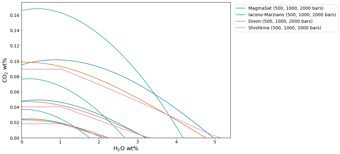
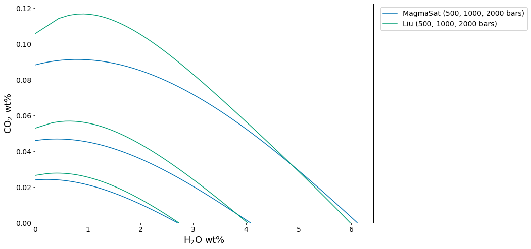
Figure 13:Isobars plotted for an alkali basalt (a) and rhyolite (b) with VESIcal for five mixed-fluid solubility models. For alkali basalt, MagmaSat, Iacono-Marziano, Dixon, and ShishkinaIdealMixing were used to create isobars at 1,200 °C. For rhyolite, MagmaSat and Liu were used to create isobars at 800 °C.
It is immediately clear from Figure 10 that major disagreement exists between these models. For the alkali basalt, MagmaSat and Dixon show the best agreement, particularly at pressures <2000 bars. However, the mismatch between these models (and, indeed, between all models) increases with pressure. The Iacono-Marziano model is calibrated for highly depolymerized alkali basalts resulting in an increased capacity of the melt to dissolve CO. That may explain why this model predicts significantly higher CO2 solubilities at XH2Ofluid values approaching 0.
The ShishkinaIdealMixing model displays nearly linear isobars, with finite solubility below ~1 wt% dissolved H2O. This is a consequence of the model calibration; the pure-H2O solubility expression of ShishkinaIdealMixing is not calibrated with any experiments at low PH2O. This results in a finite solubility at low dissolved H2O concentrations, such that the zero-pressure solubility is not zero. This produces significant model error at low but non-zero values of XH2Ofluid. Thus, we caution the user against using the ShishkinaIdealMixing model at low but non-zero XH2Ofluid or when fluids deviate far from pure H2O or pure CO2. In general, the Shishkina model should only be used for modeling pure-H2O or pure-CO2 fluids. This is discussed in more detail in Wieser et al. (2021).
The models of MagmaSat and Liu show a similar level of disagreement for H2O-CO2 solubility in the rhyolite, with Liu predicting much higher dissolved CO2 concentrations at low XH2Ofluid (<20 relative% or ~220 ppm at XH2Ofluid=0.1).
4.3Sensitivity and error analysis
To date, very few studies have compared the sensitivity of their pressure estimates to the choice of solubility model, or propagated errors inherent to measurements of volatile concentrations in melts using SIMS, FTIR and Raman Spectroscopy into an error bar in terms of saturation pressure. In contrast, VESIcal allows users to import an Excel or CSV spreadsheet with each row containing the major element and volatile contents of each inclusion, as well as a temperature at which to evaluate solubility. Using the batch calculation functions, VESIcal will automatically calculate the saturation pressure for each row, using a user-specified model. Thus, users can more easily compare results from different solubility models, to robustly assess their applicability for the system of interest. Additionally, users could load a different spreadsheet, where the CO2 and H2O concentrations are adjusted to reflect the analytical uncertainty on the instrument used, allowing error bars on the saturation pressure to be calculated for every single inclusion. The modular and open-source nature of VESIcal also allows the user to combine the code with other Python3 modules. For example, users could utilize Markov chain Monte Carlo (MCMC; e.g., the python library emcee) methods to robustly calculate error distributions for each sample. In future releases, automatic sensitivity and error analysis on datasets and calculated results may be implemented directly within VESIcal, building on existing tools within the python community.
4.4Future development
VESIcal represents the first comprehensive volatile solubility modeling tool of its kind, including the feature that VESIcal is extensible. VESIcal is written so that implementing new or yet-to-be-implemented solubility models is as simple as possible. To implement a new model, python code describing the model equations needs to be written, and this model name needs to be added to a list of model names within the code. To make this as simple as possible such that the original authors of VESIcal are not the only people who can develop the code, planned future work includes the creation of detailed instructions (including instructional videos) illustrating this process.
Likewise, new features can be added at any time, and enthusiastic members of the community who wish to help bring such features to VESIcal are very welcome. Users can contribute to VESIcal’s code, implementing new models and new features, via github (https://
4.5How to cite VESIcal and its models
To cite computations done using VESIcal, please cite this manuscript, the VESIcal version number, as well as the model(s) used. Note that if a model was not specified during calculations, the default model of MagmaSat was used and should be cited as “MagmaSat Ghiorso & Gualda, 2015”. For example: “Calculations were performed using VESIcal v. 1.0.1, Iacovino et al., 2021 with the models of Shishkina et al. (2014) and Dixon (1997, "VolatileCalc").” The web-app always runs on the most up-to-date version of the VESIcal code, but it is best practice to note if the web-app was used (“Calculations were performed using the VESIcal web-app v. 1.0.1, Iacovino et al., 2021...”). We also encourage users to be as explicit as possible as to the conditions used for modelling. This includes stating the pressure, temperature, volatile concentration, and bulk magma composition used in modelling. In the best case, VESIcal users will provide their code (e.g., as a Jupyter Notebook or .py file) along with their publication such that it can be easily replicated.
5Conclusions
VESIcal is a thermodynamic mixed-volatile solubility engine designed to meet the growing computational needs of the igneous petrology community. Seven commonly used volatile solubility models are built into VESIcal, which employs the most diversely calibrated (chemically and in P-T space) of the group, MagmaSat Ghiorso & Gualda, 2015, as the default model. VESIcal can perform five core calculations with any mixed-fluid model and three core calculations with any model (mixed-fluid, CO2-only, H2O-only). VESIcal allows for automatic calculation of large datasets and robust built-in plotting capability.
Alongside model frameworks such as ENKI, VESIcal represents an early step forward toward creating a generalized thermodynamic framework to model whole scale magmatic processes. Such a framework builds upon the key tenets of VESIcal; namely: fundamental thermodynamic underpinning; inclusion of existing modeling strategies; python powered, open-source, and extensible code base; high usability at all levels; benchmarking and testing; and power as a responsive and predictive tool.
Acknowledgments
This manuscript is dedicated to the memory of Dr. Peter Fox without whom none of this work would have been possible. We thank Peter for his encouragement of this work, his editorial handling of the manuscript, and for blazing a path for bringing executable manuscripts to AGU journals. KI and GMM were supported by the NASA Jacobs JETS Contract #NNJ13HA01C. PEW acknowledges support from a NERC DTP studentship (NE/L002507/1). The authors thank Jackie Dixon and Bob Myhill for reviews, which greatly helped strengthen this manuscript and the VESIcal code. The authors would also like to thank Mark Ghiorso, Aaron Wolf, and the ENKI team for pushing thermodynamic modeling into the future and for making this publication possible; Chelsea Allison and Giada Iacono-Marziano for discussions on their published models and how to properly implement them in VESIcal; Christy B. Till for support of KI during early coding work with MagmaSat; and presentationgo for style elements used in flowchart figures. Permission for the use of the VESIcal fox logo was graciously provided by DeviantArt user Twai.
Data Availability
The VESIcal software is open source and is hosted on github (https://
All data sets used in this manuscript are available on the VESIcal github as well as in the Supplementary Material of this manuscript. The example dataset used for worked examples in Section 3 (example_data.xlsx file; Supplemental Dataset S1) contains compositional information for basalts Tucker et al., 2019Roggensack, 2001, andesites Moore et al., 1998, rhyolites Mercer et al., 2015Myers et al., 2019, and alkaline melts (phototephrite, basaltic-trachyandesite, and basanite from Iacovino et al. (2016)). Several additional example datasets from the literature are available in the Supplement (Supplementary Datasets S2-S5; Table 4). These include experimentally produced alkaline magmas from Iacovino et al. (2016) (alkaline.xlsx), basaltic melt inclusions from Kilauea Tucker et al., 2019 and Gakkel Ridge Bennett et al., 2019 (basalts.xlsx), basaltic melt inclusions from Cerro Negro volcano, Nicaragua Roggensack, 2001 (cerro_negro.xlsx), and rhyolite melt inclusions from the Taupo Volcanic Center, New Zealand Myers et al., 2019 and a topaz rhyolite from the Rio Grande Rift Mercer et al. (2015) (rhyolites.xlsx). Where available, the calibration datasets for VESIcal models are also provided (Supplementary Datasets S6-S7).
- Tait, S., Jaupart, C., & Vergniolle, S. (1989). Pressure, gas content and eruption periodicity of a shallow, crystallising magma chamber. Earth and Planetary Science Letters, 92(1), 107–123. 10.1016/0012-821x(89)90025-3
- Blake, S. (1984). Volatile oversaturation during the evolution of silicic magma chambers as an eruption trigger. Journal of Geophysical Research, 89, 8237–8244. 10.1029/jb089ib10p08237
- Stock, M., Humphreys, M., Smith, V., Isaia, R., & Pyle, D. (2016). Late-stage volatile saturation as a potential trigger for explosive volcanic eruptions. Nature Geoscience, 9(3), 249–254. 10.1038/ngeo2639
- Stolper, E. (1982). The speciation of water in silicate melts. Geochimica et Cosmochimica Acta, 46(12), 2609–2620. 10.1016/0016-7037(82)90381-7
- Dixon, J., Stolper, E., & Holloway, J. (1995). An experimental study of water and carbon dioxide solubilities in mid-ocean ridge basaltic liquids. Part I: Calibration and solubility models. Journal of Petrology, 36, 1633–1646. 10.1093/oxfordjournals.petrology.a037267
- Moore, G., Vennemann, T., & Carmichael, I. (1998). An empirical model for the solubility of H2O in magmas to 3 kilobars. American Mineralogist, 83, 36–42. 10.2138/am-1998-1-203
- Liu, Y., Zhang, Y., & Behrens, H. (2005). Solubility of H2O in rhyolitic melts at low pressures and a new empirical model for mixed H2O-CO2 solubility in rhyolitic melts. Journal of Volcanology and Geothermal Research, 143, 219–235. 10.1016/j.jvolgeores.2004.09.019
- Iacono-Marziano, G., Morizet, Y., Trong, E., & Gaillard, F. (2012). New experimental data and semi-empirical parameterization of H2O-CO2 solubility in mafic melts. Geochimica et Cosmochimica Acta, 97, 1–23. 10.1016/j.gca.2012.08.035
- Iacovino, K., Moore, G., Roggensack, K., Oppenheimer, C., & Kyle, P. (2013). H2O-CO2 solubility in mafic alkaline magma: Applications to volatile sources and degassing behavior at Erebus volcano, Antarctica. Contributions to Mineralogy and Petrology, 166, 845–860. 10.1007/s00410-013-0877-2
- Ghiorso, M., & Gualda, G. (2015). An H2O–CO2 mixed fluid saturation model compatible with rhyolite-MELTS. Contributions to Mineralogy and Petrology, 169, 1–30. 10.1007/s00410-015-1141-8
- Papale, P., Morretti, R., & Barbato, D. (2006). The compositional dependence of the saturation surface of H2O + CO2 fluids in silicate melts. Chemical Geology, 229, 78–95. 10.1016/j.chemgeo.2006.01.013
- Bennett, E., Jenner, F., Millet, M.-A., Cashman, K., & Lissenberg, J. (2019). Deep roots for mid-ocean-ridge volcanoes revealed by plagioclase-hosted melt inclusions. Nature, 572(235). 10.1038/s41586-019-1448-0
- Dixon, J. (1997). Degassing of alkalic basalts. American Mineralogist, 82, 368–378. 10.2138/am-1997-3-415
- Shishkina, T., Botcharnikov, R., Holtz, F., Almeev, R., Jazwa, A., & Jakubiak, A. (2014). Compositional and pressure effects on the solubility of H2O and CO2 in mafic melts. Chemical Geology, 388, 112–129. 10.1016/j.chemgeo.2014.09.001
- Newman, S., & Lowenstern, J. (2002). VolatileCalc: A silicate melt-H2O-CO2 solution model written in Visual Basic for excel. Computers & Geosciences, 28, 597–604. 10.1016/s0098-3004(01)00081-4