VESIcal: An open-source thermodynamic model engine for mixed volatile (H₂O-CO₂) solubility in silicate melts
Contents
Calibration: VolatileCalc (Dixon, 1997)
This code assesses the outputs of VESIcal compared to the VolatileCalc parameterization of the Dixon (1997) model.
- Test 1 compares saturation pressures from VolatileCalc and a Excel Macro with those from VESIcal for a variety of natural compositions, and synthetic arrays.
- Test 2 compares X in the fluid phase at volatile saturation to that outputted by the Dixon Macro, and VolatileCalc
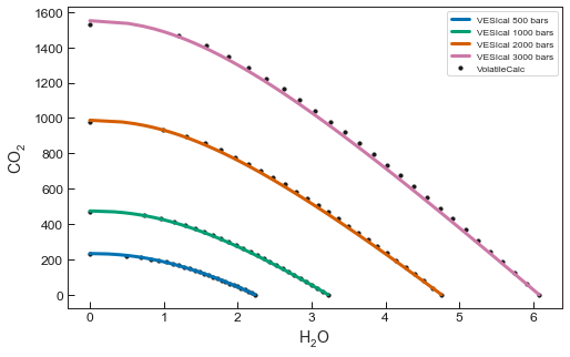
- Test 3 compares isobars with those of VolatileCalc
- Test 4 compares degassing paths
import VESIcal as v
import matplotlib.pyplot as plt
import numpy as np
import pandas as pd
from IPython.display import display, HTML
import pandas as pd
import matplotlib as mpl
import seaborn as sns
%matplotlib inline
from sklearn.linear_model import LinearRegression
from sklearn.metrics import r2_score
sns.set(style="ticks", context="poster",rc={"grid.linewidth": 1,"xtick.major.width": 1,"ytick.major.width": 1, 'patch.edgecolor': 'black'})
plt.style.use("seaborn-colorblind")
plt.rcParams["font.size"] =12
plt.rcParams["mathtext.default"] = "regular"
plt.rcParams["mathtext.fontset"] = "dejavusans"
plt.rcParams['patch.linewidth'] = 1
plt.rcParams['axes.linewidth'] = 1
plt.rcParams["xtick.direction"] = "in"
plt.rcParams["ytick.direction"] = "in"
plt.rcParams["ytick.direction"] = "in"
plt.rcParams["xtick.major.size"] = 6 # Sets length of ticks
plt.rcParams["ytick.major.size"] = 4 # Sets length of ticks
plt.rcParams["ytick.labelsize"] = 12 # Sets size of numbers on tick marks
plt.rcParams["xtick.labelsize"] = 12 # Sets size of numbers on tick marks
plt.rcParams["axes.titlesize"] = 14 # Overall title
plt.rcParams["axes.labelsize"] = 14 # Axes labels
plt.rcParams["legend.fontsize"]= 141Test 1 - Comparing saturation pressures from VESIcal to VolatileCalc and the Dixon macro
myfile = v.BatchFile('S2_Testing_Dixon_1997_VolatileCalc.xlsx')
data = myfile.get_data()
VolatileCalc_PSat=data['VolatileCalc_P'] # Saturation pressure from VolatileCalc
DixonMacro_PSat=data['DixonMacro_P'] # Saturation pressure from dixon
satPs_wtemps_Dixon= myfile.calculate_saturation_pressure(temperature="Temp", model='Dixon')
# Making linear regression
# VolatileCalc
X=VolatileCalc_PSat
Y=satPs_wtemps_Dixon['SaturationP_bars_VESIcal']
mask = ~np.isnan(X) & ~np.isnan(Y)
X_noNan=X[mask].values.reshape(-1, 1)
Y_noNan=Y[mask].values.reshape(-1, 1)
lr=LinearRegression()
lr.fit(X_noNan,Y_noNan)
Y_pred=lr.predict(X_noNan)
#X - Y comparison of pressures
fig, (ax1, ax2) = plt.subplots(1, 2, figsize = (12,5)) # adjust dimensions of figure here
ax1.set_title('Comparison of VolatileCalc and VESIcal', fontsize=14)
ax1.set_xlabel('P$_{Sat}$ VolatileCalc', fontsize=14)
ax1.set_ylabel('P$_{Sat}$ VESIcal', fontsize=14)
ax1.plot(X_noNan,Y_pred, color='red', linewidth=1)
ax1.scatter(X_noNan, Y_noNan, s=50, edgecolors='k', facecolors='silver', marker='o')
I='Intercept= ' + str(np.round(lr.intercept_, 1))[1:-1]
G='Gradient= ' + str(np.round(lr.coef_, 4))[2:-2]
R='R$^2$= ' + str(np.round(r2_score(Y_noNan, Y_pred), 4))
#one='1:1 line'
ax1.text(1000, 3700, I, fontsize=14)
ax1.text(1000, 4000, G, fontsize=14)
ax1.text(1000, 4300, R, fontsize=14)
#Dixon Macro
X=DixonMacro_PSat
Y=satPs_wtemps_Dixon['SaturationP_bars_VESIcal']
mask = ~np.isnan(X) & ~np.isnan(Y)
X_noNan=X[mask].values.reshape(-1, 1)
Y_noNan=Y[mask].values.reshape(-1, 1)
lr=LinearRegression()
lr.fit(X_noNan,Y_noNan)
Y_pred=lr.predict(X_noNan)
#X - Y comparison of pressures
ax2.set_title('Comparison of the Dixon Macro and VESIcal', fontsize=14)
ax2.set_xlabel('P$_{Sat}$ VolatileCalc', fontsize=14)
ax2.set_ylabel('P$_{Sat}$ VESIcal', fontsize=14)
ax2.plot(X_noNan,Y_pred, color='red', linewidth=1)
ax2.scatter(X_noNan, Y_noNan, s=50, edgecolors='k', facecolors='silver', marker='o')
#plt.plot([0, 4000], [0, 4000])
I='Intercept= ' + str(np.round(lr.intercept_, 1))[1:-1]
G='Gradient= ' + str(np.round(lr.coef_, 4))[2:-2]
R='R$^2$= ' + str(np.round(r2_score(Y_noNan, Y_pred), 5))
#one='1:1 line'
ax2.text(1000, 3700, I, fontsize=14)
ax2.text(1000, 4000, G, fontsize=14)
ax2.text(1000, 4300, R, fontsize=14)
ax1.set_ylim([0, 5500])
ax1.set_xlim([0, 5500])
ax2.set_ylim([0, 5500])
ax2.set_xlim([0, 5500])
plt.subplots_adjust(left=0.125, bottom=None, right=0.9, top=None, wspace=0.3, hspace=None)
ax1.text(30, 5200, 'a)', fontsize=14)
ax2.text(30, 5200, 'b)', fontsize=14)
fig.savefig('VolatileCalc_Test1a.png', transparent=True)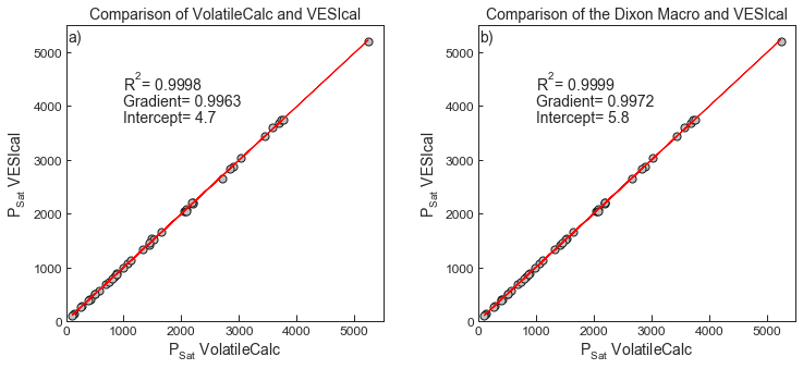
# This shows the % difference between VolatileCalc and VESIcal. The differences are similar in magnitude to those between VolatileCalc and the
# Dixon Macro
fig, (ax1, ax2, ax3) = plt.subplots(1, 3,figsize = (15,5))
font = {'family': 'sans-serif',
        'color':  'black',
        'weight': 'normal',
        'size': 20,
        }

ax1.set_xlabel('% Difference (VolatileCalc/VESIcal)', fontsize=14)
ax1.set_ylabel('# of measurements', fontsize=14)
ax1.hist(100*VolatileCalc_PSat/satPs_wtemps_Dixon['SaturationP_bars_VESIcal'])

ax2.set_xlabel('% Difference (DixonMacro/VESIcal)', fontsize=14)
ax2.set_ylabel('# of measurements', fontsize=14)
ax2.hist(100*DixonMacro_PSat/satPs_wtemps_Dixon['SaturationP_bars_VESIcal'])

ax3.set_xlabel('% Difference (DixonMacro/VolatileCalc)', fontsize=14)
ax3.set_ylabel('# of measurements', fontsize=14)
ax3.hist(100*DixonMacro_PSat/VolatileCalc_PSat)
plt.subplots_adjust(left=0.125, bottom=None, right=0.9, top=None, wspace=0.2, hspace=None)
ax1.tick_params(axis="x", labelsize=12)
ax1.tick_params(axis="y", labelsize=12)
ax2.tick_params(axis="x", labelsize=12)
ax2.tick_params(axis="y", labelsize=12)
ax3.tick_params(axis="y", labelsize=12)
ax3.tick_params(axis="x", labelsize=12)
ax1.set_xlim([97, 104])
ax2.set_xlim([98, 102])
#ax3.set_xlim([95, 104])
ax1.tick_params(direction='in', length=6, width=1, colors='k',
               grid_color='k', grid_alpha=0.5)
ax2.tick_params(direction='in', length=6, width=1, colors='k',
               grid_color='k', grid_alpha=0.5)
ax3.tick_params(direction='in', length=6, width=1, colors='k',
               grid_color='k', grid_alpha=0.5)
ax1.text(97.3, 13.7, 'a)', fontsize=14)
ax2.text(98.2, 11.7, 'b)', fontsize=14)
ax3.text(87.4, 32, 'c)', fontsize=14)
fig.savefig('VolatileCalc_Test1b.png', transparent=True)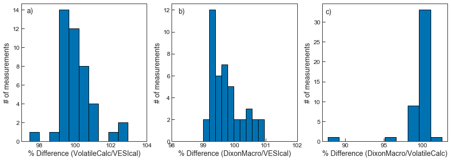
X=satPs_wtemps_Dixon['VolatileCalc_P']
Y=satPs_wtemps_Dixon['SaturationP_bars_VESIcal']
mask = (satPs_wtemps_Dixon['CO2']>0)
X_noNan=X[mask].values.reshape(-1, 1)
Y_noNan=Y[mask].values.reshape(-1, 1)
lr=LinearRegression()
lr.fit(X_noNan,Y_noNan)
Y_pred=lr.predict(X_noNan)
#X - Y comparison of pressures
fig, ax1 = plt.subplots( figsize = (10,8)) # adjust dimensions of figure here
font = {'family': 'sans-serif',
        'color':  'black',
        'weight': 'normal',
        'size': 20,
        }
ax1.set_title('Comparison of VolatileCalc and VESIcal',
        fontdict= font, pad = 15)
ax1.set_xlabel('P$_{Sat}$ VolatileCalc', fontdict=font, labelpad = 15)
ax1.set_ylabel('P$_{Sat}$ VESIcal', fontdict=font, labelpad = 15)
ax1.plot(X_noNan,Y_pred, color='red', linewidth=1)
ax1.scatter(X_noNan, Y_noNan,  s=100, edgecolors='gray', facecolors='silver', marker='o')
I='Intercept= ' + str(np.round(lr.intercept_, 3))[1:-1]
G='Gradient= '  + str(np.round(lr.coef_, 5))[2:-2]
R='R$^2$= ' +  str(np.round(r2_score(Y_noNan, Y_pred), 5))
#one='1:1 line'
plt.plot([0, 2000], [0, 2000])
ax1.text(500, 3000, I, fontsize=15)
ax1.text(500, 3500, G, fontsize=15)
ax1.text(500, 4000, R, fontsize=15)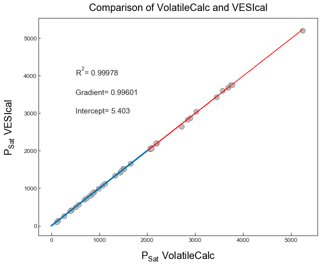
2Test 2 - Comparing X in the fluid at the saturation pressure to that calculated using VolatileCalc and the Dixon Macro
eqfluid_Dixon_VolatileCalcP = myfile.calculate_equilibrium_fluid_comp(temperature="Temp", model='Dixon', pressure = None)
eqfluid_Dixon_DixonMacroP = myfile.calculate_equilibrium_fluid_comp(temperature="Temp", model='Dixon', pressure = None)
# Making linear regression
# VolatileCalc
X=0.01*eqfluid_Dixon_VolatileCalcP['VolatileCalc_H2Ov mol% (norm)'] # VolatileCalc outputs in %
Y=eqfluid_Dixon_VolatileCalcP['XH2O_fl_VESIcal']
mask = ~np.isnan(X) & ~np.isnan(Y)
X_noNan=X[mask].values.reshape(-1, 1)
Y_noNan=Y[mask].values.reshape(-1, 1)
lr=LinearRegression()
lr.fit(X_noNan,Y_noNan)
Y_pred=lr.predict(X_noNan)
#X - Y comparison of pressures
fig, (ax1, ax2) = plt.subplots(1, 2, figsize = (12,5)) # adjust dimensions of figure here
ax1.set_xlabel('X$_{H2O}$ VolatileCalc', fontsize=14)
ax1.set_ylabel('X$_{H2O}$ VESIcal', fontsize=14)
ax1.scatter(X_noNan, Y_noNan, s=50, edgecolors='k', facecolors='silver', marker='o')
ax1.plot(X_noNan,Y_pred, color='red', linewidth=1)
I='Intercept= ' + str(np.round(lr.intercept_, 3))[1:-1]
G='Gradient= ' + str(np.round(lr.coef_, 5))[2:-2]
R='R$^2$= ' + str(np.round(r2_score(Y_noNan, Y_pred), 5))
ax1.text(0, 0.5, I, fontsize=14)
ax1.text(0, 0.6, G, fontsize=14)
ax1.text(0, 0.7, R, fontsize=14)
# Dixon Macro
X=eqfluid_Dixon_DixonMacroP['DixonMacro_XH2O']
Y=eqfluid_Dixon_DixonMacroP['XH2O_fl_VESIcal']
mask = ~np.isnan(X) & ~np.isnan(Y)
X_noNan=X[mask].values.reshape(-1, 1)
Y_noNan=Y[mask].values.reshape(-1, 1)
lr=LinearRegression()
lr.fit(X_noNan,Y_noNan)
Y_pred=lr.predict(X_noNan)
ax2.set_xlabel('X$_{H2O}$ DixonMacro', fontsize=14)
ax2.set_ylabel('X$_{H2O}$ VESIcal', fontsize=14)
ax2.plot(X_noNan,Y_pred, color='red', linewidth=1)
ax2.scatter(X_noNan, Y_noNan, s=50, edgecolors='k', facecolors='silver', marker='o')
I='Intercept= ' + str(np.round(lr.intercept_, 5))[1:-1]
G='Gradient= ' + str(np.round(lr.coef_, 5))[2:-2]
R='R$^2$= ' + str(np.round(r2_score(Y_noNan, Y_pred), 5))
ax2.text(0, 0.5, I, fontsize=14)
ax2.text(0, 0.6, G, fontsize=14)
ax2.text(0, 0.7, R, fontsize=14)
plt.subplots_adjust(left=0.125, bottom=None, right=0.9, top=None, wspace=0.3, hspace=None)
ax1.text(-0.05, 1.01, 'a)', fontsize=14)
ax2.text(-0.05, 1.01, 'b)', fontsize=14)
fig.savefig('VolatileCalc_Test2.png', transparent=True)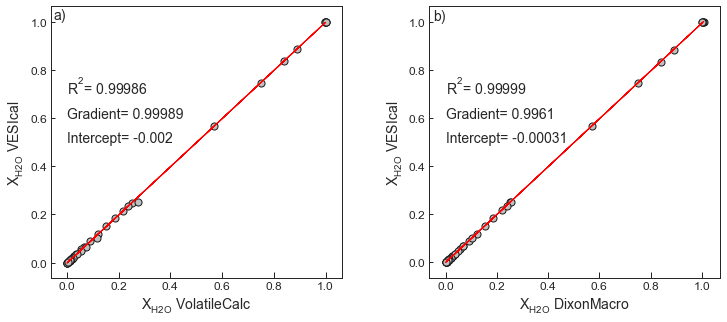
3Test 3 - Comparing Isobars to those calculated in VolatileCalc
#Loading Isobars from VolatileCalc
Isobar_output= pd.read_excel('S2_Testing_Dixon_1997_VolatileCalc.xlsx', sheet_name='Isobar_Outputs', index_col=0)
myfile_Isobar_input= v.BatchFile('S2_Testing_Dixon_1997_VolatileCalc.xlsx', sheet_name='Isobar_Comp')
data_Isobar_input = myfile_Isobar_input.data
SampleName='0'
bulk_comp= myfile_Isobar_input.get_sample_composition(SampleName, asSampleClass=True)
temperature=1200
# Calculating isobars
isobars, isopleths = v.calculate_isobars_and_isopleths(sample=bulk_comp, model='Dixon',
temperature=temperature,
pressure_list=[500, 1000, 2000, 3000],
isopleth_list=[0, 0.1, 0.2, 0.3, 0.5, 0.8, 0.9, 1],
print_status=True).resultfig, ax1 = plt.subplots(figsize = (8,5))
mpl.rcParams['axes.linewidth'] = 1
mpl.rcParams.update({'font.size': 10})
plt.scatter(Isobar_output['Wt%H2O'], Isobar_output['PPMCO2'], marker='o', s=10, label='VolatileCalc', color='k')
plt.plot(isobars.loc[isobars.Pressure==500, 'H2O_liq'], (10**4)*isobars.loc[isobars.Pressure==500, 'CO2_liq'], label='VESIcal 500 bars')
plt.plot(isobars.loc[isobars.Pressure==1000, 'H2O_liq'], (10**4)*isobars.loc[isobars.Pressure==1000, 'CO2_liq'], label='VESIcal 1000 bars')
plt.plot(isobars.loc[isobars.Pressure==2000, 'H2O_liq'], (10**4)*isobars.loc[isobars.Pressure==2000, 'CO2_liq'], label='VESIcal 2000 bars')
plt.plot(isobars.loc[isobars.Pressure==3000, 'H2O_liq'], (10**4)*isobars.loc[isobars.Pressure==3000, 'CO2_liq'], label='VESIcal 3000 bars')
plt.legend(fontsize='small')
ax1.set_xlabel('H$_2$O', fontsize=14)
ax1.set_ylabel('CO$_2$', fontsize=14)
ax1.tick_params(axis="x", labelsize=12)
ax1.tick_params(axis="y", labelsize=12)
ax1.tick_params(direction='in', length=6, width=1, colors='k',
grid_color='k', grid_alpha=0.5)
fig.savefig('VolatileCalc_Test3.png', transparent=True)