VESIcal: An open-source thermodynamic model engine for mixed volatile (H₂O-CO₂) solubility in silicate melts
Contents
Calibration: Shishkina et al. (2014)
This notebook compares the outputs from VESIcal to the Shishkina et al. (2014) Calibration dataset.
- This notebook relies on the Excel spreadsheet entitled: S7
_Testing _Shishkina _et _al _2014 .xlsx - Test 1 compares the experimental pressures in the calibration dataset of Shishkina et al. (2014) for H2O-only experiments to the saturation pressures obtained from VESIcal for the “ShishkinaWater” model.
- Test 2 compares the experimental pressures in the calibration dataset of Shishkina et al. (2014) for CO2-only experiments to the saturation pressures obtained from VESIcal for the “ShishkinaCarbon” model.
- Test 3 compares the experimental pressures for mixed H2O-CO2 bearing fluids presented in Table 2 of the main text to the saturation pressures obtained from VESIcal for the “Shishkina” model.
- Test 4 justifies the approach used in VESIcal, where cation fractions for their equation 9 are calculated ignoring H2O and CO2
import VESIcal as v
import matplotlib.pyplot as plt
import numpy as np
from IPython.display import display, HTML
import pandas as pd
import matplotlib as mpl
import seaborn as sns
from sklearn.linear_model import LinearRegression
from sklearn.metrics import r2_score
import statsmodels.api as sm
from statsmodels.sandbox.regression.predstd import wls_prediction_std
%matplotlib inline
sns.set(style="ticks", context="poster",rc={"grid.linewidth": 1,"xtick.major.width": 1,"ytick.major.width": 1, 'patch.edgecolor': 'black'})
plt.style.use("seaborn-colorblind")
plt.rcParams["font.size"] =12
plt.rcParams["mathtext.default"] = "regular"
plt.rcParams["mathtext.fontset"] = "dejavusans"
plt.rcParams['patch.linewidth'] = 1
plt.rcParams['axes.linewidth'] = 1
plt.rcParams["xtick.direction"] = "in"
plt.rcParams["ytick.direction"] = "in"
plt.rcParams["ytick.direction"] = "in"
plt.rcParams["xtick.major.size"] = 6 # Sets length of ticks
plt.rcParams["ytick.major.size"] = 4 # Sets length of ticks
plt.rcParams["ytick.labelsize"] = 12 # Sets size of numbers on tick marks
plt.rcParams["xtick.labelsize"] = 12 # Sets size of numbers on tick marks
plt.rcParams["axes.titlesize"] = 14 # Overall title
plt.rcParams["axes.labelsize"] = 14 # Axes labels
plt.rcParams["legend.fontsize"]= 140.1Test 1 and 2 - comparing saturation pressures to experimental pressures
myfile_CO2 = v.BatchFile('S7_Testing_Shishkina_et_al_2014.xlsx', sheet_name='CO2') # Loading Carbon calibration dataset
satPs_wtemps_Shish_CO2= myfile_CO2.calculate_saturation_pressure(temperature="Temp", model='ShishkinaCarbon') # Calculating saturation pressures
myfile_H2O = v.BatchFile('S7_Testing_Shishkina_et_al_2014.xlsx', sheet_name='H2O') # Loading Water calibration dataset
satPs_wtemps_Shish_H2O= myfile_H2O.calculate_saturation_pressure(temperature="Temp", model='ShishkinaWater') # Calculating Saturation pressures
######################## H2O only experiments
# This calculating a linear regression, and plots experimental pressures vs. saturation pressures for the Water calibration dataset
X_Test1=satPs_wtemps_Shish_H2O['Press']
Y_Test1=satPs_wtemps_Shish_H2O['SaturationP_bars_VESIcal']
mask_Test1 = (X_Test1>-1) & (Y_Test1>-1) # This gets rid of Nans
X_Test1noNan=X_Test1[mask_Test1].values.reshape(-1, 1)
Y_Test1noNan=Y_Test1[mask_Test1].values.reshape(-1, 1)
lr=LinearRegression()
lr.fit(X_Test1noNan,Y_Test1noNan)
Y_pred_Test1=lr.predict(X_Test1noNan)
fig, (ax1, ax2) = plt.subplots(1,2, figsize=(12,5)) # adjust dimensions of figure here
ax1.plot(X_Test1noNan,Y_pred_Test1, color='red', linewidth=0.5, zorder=1) # This plots the best fit line
ax1.scatter(satPs_wtemps_Shish_H2O['Press'], satPs_wtemps_Shish_H2O['SaturationP_bars_VESIcal'], s=50, edgecolors='k', facecolors='silver', marker='o', zorder=5)
# This bit plots the regression parameters on the graph
I='Intercept= ' + str(np.round(lr.intercept_, 1))[1:-1]
G='Gradient= ' + str(np.round(lr.coef_, 3))[2:-2]
R='R$^2$= ' + str(np.round(r2_score(Y_Test1noNan, Y_pred_Test1), 3))
ax1.text(3000, 1500, R, fontsize=14)
ax1.text(3000, 1000, G, fontsize=14)
ax1.text(3000, 500, I, fontsize=14)
################### CO2 experiments
X_Test2=satPs_wtemps_Shish_CO2['Press']
Y_Test2=satPs_wtemps_Shish_CO2['SaturationP_bars_VESIcal']
mask_Test2 = (X_Test2>-1) & (Y_Test2>-1) # This gets rid of Nans
X_Test2noNan=X_Test2[mask_Test2].values.reshape(-1, 1)
Y_Test2noNan=Y_Test2[mask_Test2].values.reshape(-1, 1)
lr=LinearRegression()
lr.fit(X_Test2noNan,Y_Test2noNan)
Y_pred_Test2=lr.predict(X_Test2noNan)
ax2.plot(X_Test2noNan,Y_pred_Test2, color='red', linewidth=0.5, zorder=1) # This plots the best fit line
ax2.scatter(satPs_wtemps_Shish_CO2['Press'], satPs_wtemps_Shish_CO2['SaturationP_bars_VESIcal'], s=50, edgecolors='k', facecolors='silver', marker='o', zorder=5)
# This bit plots the regression parameters on the graph
I='Intercept= ' + str(np.round(lr.intercept_, 2))[1:-1]
G='Gradient= ' + str(np.round(lr.coef_, 3))[2:-2]
R='R$^2$= ' + str(np.round(r2_score(Y_Test2noNan, Y_pred_Test2), 2))
ax2.text(4000, 500, I, fontsize=14)
ax2.text(4000, 1000, G, fontsize=14)
ax2.text(4000, 1500, R, fontsize=14)
ax1.set_xlabel('Experimental Pressure (bar)', fontsize=14)
ax1.set_ylabel('P$_{Sat}$ VESIcal (bar)', fontsize=14)
ax2.set_xlabel('Experimental Pressure (bar)', fontsize=14)
ax2.set_ylabel('P$_{Sat}$ VESIcal (bar)', fontsize=14)
ax1.set_xticks([0, 2000, 4000, 6000, 8000, 10000])
ax1.set_yticks([0, 2000, 4000, 6000, 8000, 10000])
ax2.set_xticks([0, 2000, 4000, 6000, 8000, 10000])
ax2.set_yticks([0, 2000, 4000, 6000, 8000, 10000])
ax1.set_xlim([-200, 6500])
ax1.set_ylim([-200, 6500])
ax2.set_xlim([-200, 8000])
ax2.set_ylim([-200, 8000])
plt.subplots_adjust(left=0.125, bottom=None, right=0.9, top=None, wspace=0.3, hspace=None)
ax1.text(-150, 6200, 'a)', fontsize=14)
ax2.text(-150, 7600, 'b)', fontsize=14)
ax1.set_title('H$_{2}$O-only', fontsize=14)
ax2.set_title('CO$_2$-only', fontsize=14)
fig.savefig('Shishkina_Test1and2.png', transparent=True)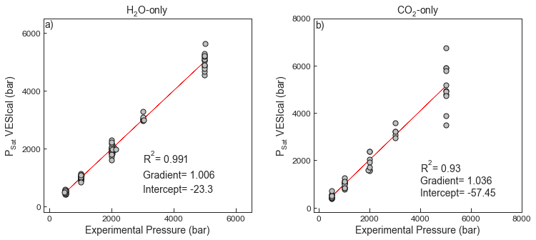
0.2Test 3 - Mixed H2O - CO2 experiments from Table 2 in the text.
- We show the regression for experimental pressure vs. saturation pressure calculated in VESIcal for all data, and data with experimental pressures <4000 bars (to remove the most scattered datapoints).
myfile_Comb = v.BatchFile('S7_Testing_Shishkina_et_al_2014.xlsx', sheet_name='Table2_Text') # Loads experimental data from Table 2
satPs_wtemps_Shish_Comb= myfile_Comb.calculate_saturation_pressure(temperature="Temp", model='ShishkinaIdealMixing') # Calculates saturation pressures for these compositions + tempts
######################## H2O only experiments
X_Test3b=satPs_wtemps_Shish_Comb['Press']
Y_Test3b=satPs_wtemps_Shish_Comb['SaturationP_bars_VESIcal']
mask_Test3b = (X_Test3b>-1) & (Y_Test3b>-1) # This gets rid of Nans
X_Test3bnoNan=X_Test3b[mask_Test3b].values.reshape(-1, 1)
Y_Test3bnoNan=Y_Test3b[mask_Test3b].values.reshape(-1, 1)
lr=LinearRegression()
lr.fit(X_Test3bnoNan,Y_Test3bnoNan)
Y_pred_Test3b=lr.predict(X_Test3bnoNan)
fig, (ax1, ax2) = plt.subplots(1,2, figsize=(12,5)) # adjust dimensions of figure here
ax1.plot(X_Test3bnoNan,Y_pred_Test3b, color='red', linewidth=0.5, zorder=1) # This plots the best fit line
ax1.scatter(satPs_wtemps_Shish_Comb['Press'], satPs_wtemps_Shish_Comb['SaturationP_bars_VESIcal'], s=50, edgecolors='k', facecolors='silver', marker='o', zorder=5)
# This bit plots the regression parameters on the graph
I='Intercept= ' + str(np.round(lr.intercept_, 1))[1:-1]
G='Gradient= ' + str(np.round(lr.coef_, 3))[2:-2]
R='R$^2$= ' + str(np.round(r2_score(Y_Test3bnoNan, Y_pred_Test3b), 3))
ax1.text(3000, 1500, R, fontsize=14)
ax1.text(3000, 1000, G, fontsize=14)
ax1.text(3000, 500, I, fontsize=14)
################### CO2 experiments
X_Test3=satPs_wtemps_Shish_Comb['Press']
Y_Test3=satPs_wtemps_Shish_Comb['SaturationP_bars_VESIcal']
mask_Test3 = (X_Test3>-1) & (Y_Test3>-1) &(X_Test3<4000) # This gets rid of Nans
X_Test3noNan=X_Test3[mask_Test3].values.reshape(-1, 1)
Y_Test3noNan=Y_Test3[mask_Test3].values.reshape(-1, 1)
lr=LinearRegression()
lr.fit(X_Test3noNan,Y_Test3noNan)
Y_pred_Test3=lr.predict(X_Test3noNan)
ax2.plot(X_Test3noNan,Y_pred_Test3, color='red', linewidth=0.5, zorder=1) # This plots the best fit line
ax2.scatter(satPs_wtemps_Shish_Comb['Press'], satPs_wtemps_Shish_Comb['SaturationP_bars_VESIcal'], s=50, edgecolors='k', facecolors='silver', marker='o', zorder=5)
# This bit plots the regression parameters on the graph
I='Intercept= ' + str(np.round(lr.intercept_, 2))[1:-1]
G='Gradient= ' + str(np.round(lr.coef_, 3))[2:-2]
R='R$^2$= ' + str(np.round(r2_score(Y_Test3noNan, Y_pred_Test3), 2))
ax2.text(2000, 100, I, fontsize=14)
ax2.text(2000, 400, G, fontsize=14)
ax2.text(2000, 700, R, fontsize=14)
ax1.set_xlabel('Experimental Pressure (bar)', fontsize=14)
ax1.set_ylabel('P$_{Sat}$ VESIcal (bar)', fontsize=14)
ax2.set_xlabel('Experimental Pressure (bar)', fontsize=14)
ax2.set_ylabel('P$_{Sat}$ VESIcal (bar)', fontsize=14)
ax1.set_xticks([0, 2000, 4000, 6000, 8000, 10000])
ax1.set_yticks([0, 2000, 4000, 6000, 8000, 10000])
ax2.set_xticks([0, 2000, 4000, 6000, 8000, 10000])
ax2.set_yticks([0, 2000, 4000, 6000, 8000, 10000])
ax1.set_xlim([-200, 8000])
ax1.set_ylim([-200, 8000])
ax2.set_xlim([-200, 4000])
ax2.set_ylim([-200, 4000])
plt.subplots_adjust(left=0.125, bottom=None, right=0.9, top=None, wspace=0.3, hspace=None)
ax1.text(-150, 7600, 'a)', fontsize=14)
ax2.text(-150, 3800, 'b)', fontsize=14)
ax1.set_title('All Experiments', fontsize=14)
ax2.set_title('Experimental Pressure < 4000 bars)', fontsize=14)
fig.savefig('Shishkina_Test3.png', transparent=True)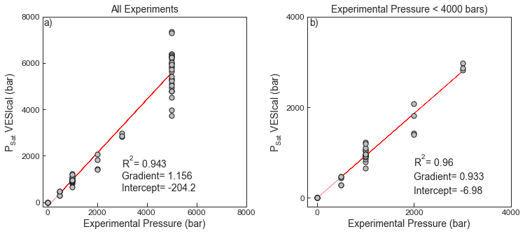
0.3Test 4 - Intepretation of "atomic fractions of cations in Equation 9.
- We can only recreate the chemical data for cation fractions shown in their Fig. 7a if the “atomic fractions of cations” are calculated excluding volatiles. Including atomic proportions including H2O and CO2 results in a significantly worse fit to experimental data for the ShishkinaWater model shown in test 2. The choice of normalization doesn’t affect the results for the CO2 model, where the compositional dependence is expressed as a fraction
# Removed CO2 and H2O
oxides = ['SiO2', 'TiO2', 'Al2O3', 'Fe2O3', 'Cr2O3', 'FeO', 'MnO', 'MgO', 'NiO', 'CoO', 'CaO', 'Na2O', 'K2O', 'P2O5']
oxideMass = {'SiO2': 28.085+32, 'MgO': 24.305+16, 'FeO': 55.845+16, 'CaO': 40.078+16, 'Al2O3': 2*26.982+16*3, 'Na2O': 22.99*2+16,
			 'K2O': 39.098*2+16, 'MnO': 54.938+16, 'TiO2': 47.867+32, 'P2O5': 2*30.974+5*16, 'Cr2O3': 51.996*2+3*16,
			 'NiO': 58.693+16, 'CoO': 28.01+16, 'Fe2O3': 55.845*2+16*3}
CationNum = {'SiO2': 1, 'MgO': 1, 'FeO': 1, 'CaO': 1, 'Al2O3': 2, 'Na2O': 2,
			 'K2O': 2, 'MnO': 1, 'TiO2': 1, 'P2O5': 2, 'Cr2O3': 2,
			 'NiO': 1, 'CoO': 1, 'Fe2O3': 2}
Normdata = myfile_H2O.get_data(normalization="additionalvolatiles")for ind,row in Normdata.iterrows():
for ox in oxides:
Normdata.loc[ind, ox + 'molar']=((row[ox]*CationNum[ox])/oxideMass[ox]) # helps us get desired column name with its actual name, rather than its index. If by number, do by iloc.
#oxide_molar[ind, ox]=ox+'molar'
Normdata.loc[ind,'sum']=sum(Normdata.loc[ind, ox+'molar'] for ox in oxides)
for ox in oxides:
Normdata.loc[ind, ox + 'norm']=Normdata.loc[ind, ox+'molar']/Normdata.loc[ind, 'sum']
# helps us get desired column name with its actual name, rather than its index. If by number, do by iloc.
Normdata.head()Loading...
### Comparison of these cation fractions to those shown in their Fig. 7afig, ax1 = plt.subplots(figsize = (10,8)) # adjust dimensions of figure here
font = {'family': 'sans-serif',
'color': 'black',
'weight': 'normal',
'size': 20,
}
plt.xlim([0, 0.25])
plt.ylim([1, 13])
plt.title('Calculated using VESIcal')
plt.scatter(Normdata['Na2Onorm']+Normdata['K2Onorm'], Normdata['H2O'], edgecolor='k', facecolor='b', s=50, label='Normalized')
plt.xlabel('Na+K')
plt.ylabel('H$_2$O')
plt.legend()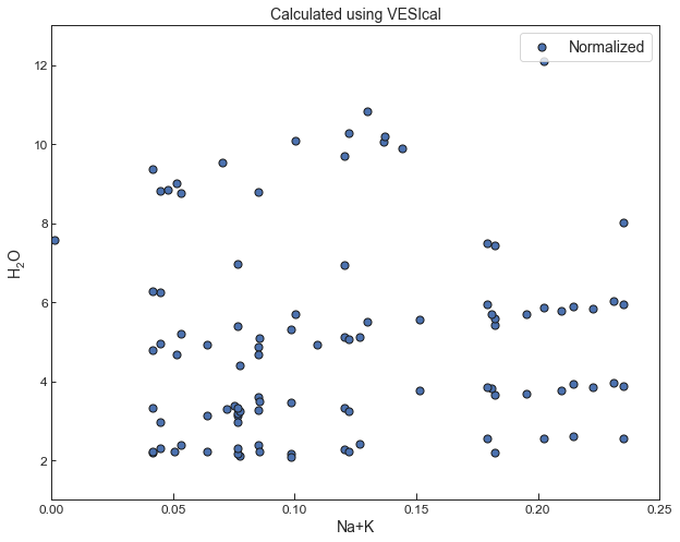
1Their graph below

- Shishkina, T., Botcharnikov, R., Holtz, F., Almeev, R., Jazwa, A., & Jakubiak, A. (2014). Compositional and pressure effects on the solubility of H2O and CO2 in mafic melts. Chemical Geology, 388, 112–129. 10.1016/j.chemgeo.2014.09.001